This study presents a recursive biomechanical model that validates that spiral phyllotaxis can be explained solely by Newtonian mechanics, without invoking additional forces or interactions. The model conceptualizes phyllotactic elements as expanding, non-deformable circles, driven by two primary forces: growth pressure, resulting from their continuous expansion, and outside pressure, arising from surrounding medium resistance. Results demonstrate that spiral structures emerge naturally, with patterns corresponding predominantly to Fibonacci and Lucas sequences. The computational implementation of the model demonstrates its capacity to produce biologically realistic patterns and reveals key insights into the dynamics of pattern formation, such as the stabilization of divergence angles and the emergence of densely packed structures. The study includes step-by-step video demonstrations and functional program code, allowing independent verification by researchers.

• Spiral Phyllotaxis

• Morphogenesis

• Fibonacci Sequence

• Dynamic Modeling

• Biomechanical Model

Rozin B, Rozin N (2025) Proof of a Recursive Biomechanical Model of Flat Spiral Phyllotaxis Morphogenesis. Int J Plant Biol Res 13(1): 1143.

Basic Terminology

• Phyllotaxis (from the Greek — leaf and táxis — arrangement): refers to the structured, often helical, periodic, and symmetrical growth patterns observed in botanical structures. These formations, exhibiting intrinsic mathematical properties, are commonly known as phyllotactic patterns.

• Primordium (plural primordia): a discrete biological entity (seed, seed, leafmagi, petal, shoot) of a phyllotactic pattern.

• Parastichy (plural parastichies): identifiable right- or left-handed spiral formed by primordia.

• The parastichy index: The numerical count of parastichies with the same twist.

• Fibonacci phyllotaxis: A pattern of spiral phyllotaxis where parastichies indexes are equal to the Fibonacci numbers (Figure 1).

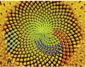
Figure 1: Planar spiral phyllotaxis in sunflower at inflorescence with a visible parastichy index of (21, 34, 55).

• Genetic spiral: An imaginary spiral that sequentially passes through all primordia.

• Divergence angle: The smaller angle between two consecutive primordia, typically aligning with the golden angle 2π/τ2 in Fibonacci phyllotaxis.

• Planar spiral phyllotaxis: A pattern observed in a flat or convex inflorescence, such as a sunflower head, where multiple spiral families coexist. (Figure 1).

• Element of a phyllotactic pattern (EPP, plural EPPs,): a mathematical abstraction of a primordium, often represented as a circle or disk in 2D models.

• EPP(i): EPP number i.

• Recurrent sequence: an integer sequence series formed by the recurrence formula Gn = Gn–1 + Gn–2 with initial terms {G1 ,G2 }. Moreover  .does not depend on the initial terms.

• Fibonacci sequence (or Fibonacci numbers): an integer recurring series with initial terms {1,1} ({0,1} or {1,2}).

• Fibonacci phyllotaxis: A pattern of spiral phyllotaxis in which parastichies indexes is equal to the Fibonacci numbers (Figure 1).

• The generating recurrent sequence: a recurrent sequence whose elements serve as parastichy indices in a given pattern.

• The phyllotaxis rises: the visual transition from a pair of parastichies with the index (Fi-1 , Fi ) to (Fi , F_ i+1 ) , a defining feature of spiral phyllotaxis.

Philosophical Aspects of Phyllotaxis

Unlike a plant, which represents a continuous biological entity, a phyllotactic pattern is composed of discrete elements known as primordia. The conceptual difference between the plant as a whole and individual primordia led [1], to define phyllotaxis morphogenesis as the process emergence discrete structures from a continuous system. This perspective implies that the morphogenesis of phyllotaxis patterns is fundamentally distinct from that of other plant structures, such as roots, leaves, or stems.

The question “Why do we perceive parastichies?” was addressed by [2], who proposed that human perception subconsciously groups adjacent primordia into pseudo structures, akin to how stars are mentally grouped into constellations. This effect is demonstrated in Video 1 https://youtu.be/ZOeF8zSulW0 [3], where stretching or compressing a cylindrical phyllotactic pattern causes EPPs to visually merge into parastichies (straight lines) before disassembling again.

Mathematical Aspects of Phyllotaxis

The fundamental relationship between recursive sequences and the golden ratio can be illustrated using a classical mathematical problem:

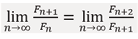
Problem: need to computelime  where the terms Fn and Fn+1 are defined by the recursive relation:

Fn+2 = Fn+1 +Fn (1)

with real initial conditions F1 >0 and F2 >0

Solution: divide both sides of the recurrence relation (1) by Fn+1

From the properties of limits:

Let us denotelim  and substitute into (1): τ=1+1/τ .

Substituting into the equation above yields the quadratic equation τ2 - τ - 1 = 0, whose positive root corresponds to the golden ratio:

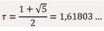
This result demonstrates that the limit of the ratio of consecutive terms in any recurrent sequence is independent of initial conditions.

Furthermore, any term of an arbitrary recurrence sequence can be expressed in terms of the Fibonacci sequence with initial values {1,2}, which serves as the fundamental recurrence sequence [2]:

Gn = Fn-2 G2 + Fn-3 G1

Modern science considers a plant as a biological object consisting of many cells between which various physical and chemical processes occur. These processes are adequately described by statistical and differential integral mathematical tools. Therefore, a significant number of researchers employ these well-tested mathematical methods to construct models of phyllotaxis morphogenesis. However, Fibonacci numbers do not arise as basic constants, either in statistics or in differential integral calculus, as, for example, the constant arises in trigonometry or in differential-integral calculus. As argued by Rozin [2], Fibonacci numbers only arise in the solution of problems involving recursion. This observation has led to the hypothesis that the morphogenesis of spiral phyllotaxis is inherently a recursive process.

Static Model

A static model represents a phyllotactic pattern as a structured arrangement of discrete elements (EPPs).

The sunflower inflorescence (Figure 1) is a striking example of flat spiral phyllotaxis, where the primordia are achenes. In Figure 1, several families of parastichies formed by achenes are visible, with the number of spirals in each family precisely corresponding to one of the Fibonacci numbers. When ignoring the visible spirals, it becomes evident from Figure 1 that the mutual arrangement of achenes closely resembles Axial, Point, and Circular symmetry. From an analysis of this quasi symmetry, Braun [4] and Schimper [5], proposed that it might be possible to trace a spiral through all primordia and number these discrete elements in accordance with their increasing distance from the center of the spiral. This ingenious hypothesis laid the foundation for mathematical phyllotaxis, and this quasi-symmetry was named Spiral Symmetry [6].

Contemporary research primarily focuses on the mechanisms underlying spiral pattern formation, emphasizing the spatial arrangement of primordia [2,7 10]. In [2], a mathematical analysis of the static model of spiral phyllotaxis led to the following key insights:

• The centers of EPPs in spiral phyllotaxis lie at the intersections of two counter-rotating genetic spirals, forming a Double Helix Model.

• Parastichies are perceptual artifacts that group adjacent EPPs into visually spiral-like pseudo objects.

These findings yielded novel quantitative and qualitative relationships, some of which are used in this study:

• The parameters defining a static spiral phyllotactic model are categorized into linear (genetic spiral shape, EPP diameter, Plastochrone ratio R) and angular (divergence angle, visible parastichy indices, inter-parastichy angles).

• The divergence angle in a spiral phyllotactic pattern is determined by non-multiplicative recurrence sequences with initial values {G1 , G2 }, where 1 < G1 ; 2G1 ≤ G2 ; gcd(G1 , G2 ) = 1; G1 , G2 , A1 , A2 ∈ N. The divergence angle can be calculated from the system of equations:

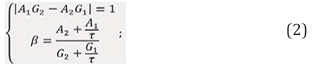
• the visual phenomenon of “The phyllotaxis rise” is observed if the genetic spiral has the form of an exponential spiral, and not a logarithmic one as it was previously thought;

• if the static model of the pattern is built on the exponential genetic spiral, then the distance from EPP(i) to the center of the pattern will be equal to:

L(i)=iv (3)

and the diameter of EPP(i) is calculated as:

Video 2 https://youtu.be/9H7Nf6BjDaA [11], shows how the static model of the pattern changes when the parameter ???? = 0.5÷3 changes, while the divergence angle and indices of visible parastichies remain unchanged. It is established that the Archimedean spiral represents a specific case of the exponential spiral with ν = 1, thus for a static model based on an Archimedean spiral, the following relationships hold: L(i)=i and . Prior to Rozin [2], this latter formula was known as [8].

Overview of Dynamic Models

In Rozin [11], four primary types of dynamic models describing the morphogenesis of phyllotaxis patterns were identified: biochemical, a model based on “Hofmeister rule”, bioinformatic, and biomechanical.

Biochemical model: A major proponent of the biochemical approach was Alan Turing, one of the most influential mathematicians of the modern era. In his seminal work [12], he described self-organization processes in matter through self-oscillating chemical reactions described by second-order differential equations. Turing was particularly interested in the phenomenon of phyllotaxis and attempted to model its morphogenesis using the same mathematical framework. His unfinished manuscript published posthumously [13], explored the possibility that Fibonacci spiral patterns in plants arise as a consequence of self-oscillating chemical reactions.

Counterargument: As previously discussed, Fibonacci numbers do not naturally emerge from second-order differential equations, casting doubt on the viability of this approach as a complete explanation for phyllotaxis morphogenesis. (2)

The criticism of “Hofmeister rule”: Figure 2A from [8], depicts an early stage of phyllotactic pattern formation in sunflower inflorescence. In the center of the inflorescence (a circle with a radius of 2/3 of the total inflorescence radius), no protuberances are observed.

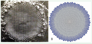
Figure 2: (?) Micrograph taken by J. H. Palmer using a scanning electron microscope [8]. Reproduced with permission from The Licensor through PLSclear. (B) Phyllotaxis pattern for 2000 elements, obtained similarly to the method demonstrated in Video 3 https://youtu.be/sJFrB7TnqPc [1].

However, within an outer ring of thickness 1/3 of the inflorescence radius, over 300 primordia are distinctly visible, forming paired parastichies with indices (55, 89).

Hofmeister [14], while observing such early stages of morphogenesis, noted that new protuberances (proprimordia) appear at the boundary between the outer and inner rings, suggesting that pattern formation from the periphery toward the center. Based on these observations, he formulated the “Hofmeister rule”, which postulates that a new primordium forms at the point farthest from existing ones.

Jean [8], describes the phyllotaxis morphogenesis model, which is based on the analysis of this micrograph: “Showing the process of floret initiation proceeding toward the center on the generative front with a remarkable degree of symmetry”. Ibid: “the primordial florets are initiated in rapid succession from the periphery to the center of the apex”. That is, Jean [8], suggests that under the influence of a certain mysterious mechanism, primordia “initiated” from the outer edge to the center. Moreover, divergence angle is maintained with the highest accuracy and the process itself is not subject to probabilistic deviations.

Counterargument: This explanation is reminiscent of the humorous statement that “a nuclear bomb always hits the epicenter of the explosion.” In biological systems, particularly those in living organisms, stochastic deviations are inevitable. Attempts to explain Hofmeister’s rule and the absence of visible primordia in the center of young inflorescences have led to numerous hypotheses based on forces not found in other phenomena of living nature, such as standing waves or interactions that contradict classical physics [15-20].

According to the authors, these issues stem from a misinterpretation of causality in the “Hofmeister rule”: a new primordium does not physically emerge but rather transitions from an invisible to a visible state.

Despite its speculative nature, the Hofmeister rule contains a kernel of truth: primordia located on the periphery of the inflorescence are older than those near the center. The age of a primordium is directly proportional to its distance from the center. Rozin [1,2] proposed an alternative explanation for the Hofmeister rule as a visual phenomenon, where each primordium undergoes an initial invisible stage before becoming visible (Video 3 https://youtu.be/sJFrB7TnqPc [1]). The validity of this hypothesis can be assessed by comparing Figure 2A and 2B.

Bioinformatic models and the role of auxin in phyllotaxis morphogenesis: A dominant contemporary hypothesis attributes the emergence of Fibonacci phyllotactic patterns to the role of auxin (a plant growth hormone) in conveying positional information for new primordium formation [21-25]. This proposed mechanism aligns with the Hofmeister rule. 

Counterargument: If auxin were the primary driver of phyllotaxis morphogenesis, artificially increasing its concentration should lead to an abnormal proliferation of primordia, disrupting the spiral pattern. However, experimental data show that auxin supplementation instead induces enhanced growth of pre-existing primordia, without generating new ones [26].

According to the authors, the informational role of auxin has been misinterpreted due to an incorrect construction of cause-and-effect relationships. Specifically, the increase in auxin concentration is a consequence of the primordium’s growth process during its transition from an invisible to a visible state, rather than a determinant of its location or emergence.

Prerequisites for the Biomechanical model: The foundations of a mechanical approach to phyllotaxis morphogenesis were established by Bravais & Bravais [27], and later developed by Church [7], Mitchinson [28], Jean [8], Niklas [29,30], and Lee & Levitov [31]. A key contribution came from Adler [32-34], who formulated the Contact Pressure Model. Researchers following Adler’s work (Vogel [35], Roberts [36-38]; Ridley [39,40], Douady & Couder [41], Hellwig et al. [42]), sought to develop models that generate spiral patterns with a constant divergence angle. However, these models presupposed the golden angle rather than deriving it as an emergent property. For example, Ridley [39], explicitly placed each new primordium at a fixed angular offset from its predecessor.

For the sake of fairness, it should be noted that the illustrations and videos from Rozin [1-3,11], were also generated using program code that incorporates the golden angle. However, these illustrations and videos serve only as explanations or visual representations of the expected results of the model’s operation and do not constitute the dynamic model itself. Building on Adler’s Contact Pressure Model, Rozin [2], proposed a recursive algorithm to transition from a phyllotactic pattern with N EPPs to a pattern with N+1 EPPs. This algorithm serves as a fundamental prerequisite for a dynamic model of spiral phyllotaxis morphogenesis:

• each new EPP appears at the center of the inflorescence at regular intervals;

• each EPP continuously grows;

• the increasing size of each EPP generates mechanical pressure on neighboring EPPs. The resultant force vector is directed outward from the center, causing each EPP to move radially outward;

• due to the rectilinear movement of each EPP from the center of the inflorescence, the divergence angle remains constant.

The operation of this recursive algorithm is explained in Video 4 https://youtu.be/nqOuWhGp82w [1]. Using this recursive algorithm [1], analytically demonstrated that if three families of parastichies (Q, R, and S from Figure 3) are observed in a pattern, their indices are consecutive terms of a recursive series (Q + R = S).

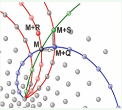
Figure 3: Phyllotaxis pattern explaining Q+R=S [3].

Cylindrical Phyllotaxis

Another important issue is the morphogenesis of cylindrical phyllotaxis. Unlike the spiral phyllotaxis, in cylindrical phyllotaxis all EPPs are of the same size. This has led many researchers [8, 27, 44-46], to falsely assume that it would be easier to construct a morphogenesis model for cylindrical phyllotaxis patterns since they have one less parameter, namely the growth function of EPPs.

Counterargument: A distinctive feature of spiral cylindrical phyllotaxis patterns observed in nature is that the opposing pair of parastichies intersect at a right angle [2,8,11]. On the other hand, it is well known that the optimal dense packing of spheres or disks of the same size is the Hexagonal Close-Packed (HCP) arrangement, which exhibits a 60-degree angle between visible “parastichies” (Figure 4).

Figure 4: Hexagonal Close-Packed (HCP) and its visible “parastichies.

The fact that the angle between the opposing parastichy in spiral cylindrical phyllotaxis is a right angle indicates that this packing of EPPs is not dense, suggesting a more complex morphogenetic process.

Rozin [2,11], hypothesized that cylindrical spiral phyllotaxis originates directly from a flat spiral pattern. According to this model, after the establishment of a flat phyllotactic pattern with a constant divergence angle, the apical center of the inflorescence gradually moves perpendicularly to the plane of the pattern. As this movement occurs, EPPs shift outward, forming a cylindrical arrangement while preserving the divergence angle and visible parastichy indices (Video 5 https://youtu.be/tzkj8FuNTPw [11]). This 3D transformation occurs exclusively under the influence of mechanical forces, without requiring additional biochemical or informational factors.

The validity of the biomechanical model for spiral cylindrical phyllotaxis morphogenesis is supported by the strong visual correspondence between the natural cylindrical structures observed in Figure 5 and the simulated pattern in Figure 6.

Figure 5: Micrograph of a Norway spruce bud (courtesy of Rolf Rutishauser).

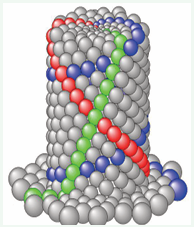
Figure 6: Final frame from Video 5 [11].

Recursive Biomechanical Model

The objective of this study is to demonstrate that the morphogenesis of flat spiral phyllotaxis patterns can be adequately described by simple mechanical interactions that do not go beyond classic physics. This will be proven by the results of testing a recursive biomechanical model. In this model, the Element of a phyllotactic pattern (EPP) is represented by the simplest object - a non-deformable circle, whose diameter increases continuously according to Formula 4. The increase in the size of the EPP creates pressure on other EPPs. EPPs press on each other, resulting in their movement according to Newton’s third law. The mechanical interaction will henceforth be referred to as growth pressure.

During the formation stage of a real inflorescence, it is evident that the structure does not develop in a vacuum but is instead surrounded by a dense and viscous plant matrix. As the inflorescence expands, it exerts force against this surrounding medium, which in turn generates a counteracting pressure directed toward the center of the inflorescence. This opposing force will be termed outside pressure.

Thus, two primary mechanical forces drive the morphogenesis of spiral phyllotaxis:

•  Growth pressure, resulting from the continuous expansion of each EPP;
•  Outside pressure, exerted by the resistance of the surrounding plant matrix.

The recursive biomechanical model of spiral phyllotaxis morphogenesis can be formalized as a recursive process wherein:

• each new EPP emerges in the space between three preceding EPPs at equal intervals at that interval representing the model step;
• each EPP undergoes continuous expansion as described by Formula 4;
• The increasing size of each EPP generates growth pressure on adjacent EPPs;
• the surrounding medium exerts outside pressure on all EPPs, directed toward the center of the structure;
• each EPP moves under the combined influence of growth pressure and outside pressure.

Expected Results

Given that the recursive biomechanical model incorporates two primary mechanical forces, the model’s behavior is expected to depend on two key parameters:

• the growth rate parameter for EPP diameter expansion, denoted as ν from Formula 4;
• the Coefficient of Outside Pressure (COP) per model step.

To evaluate the model, the authors developed a computational program biomodel_statistic in C#, which step-by-step calculates the coordinates and radii of each EPP for given ν and COP. After a predefined number of steps, the program calculates the visible parastichies index, divergence angle and its standard deviation, while also generating graphical representations resulting patterns. The outputs for various combinations of ν and COP serve as the basis for analyzing the model’s behavior.

In addition to numerical analysis, visual observation of the stepwise morphogenesis process is of interest. To facilitate this, biomodel_statistic was adapted into biomodel_video, which generates sequential graphical frames illustrating the model’s progression. These frames can be compiled into a video, enabling dynamic visualization other recursive biomechanical model over time.

The authors aimed to develop the simplest and most transparent program code possible, ensuring that any researcher with basic programming knowledge can verify the code’s fidelity to the stated algorithm. The model contains no pre-programmed mechanisms generating Fibonacci numbers or the golden angle. Moreover, researchers are encouraged to modify V and ???, or even alter the algorithm, to conduct independent analyses of the recursive biomechanical model.

Appendix A provides the full biomodel_statistic source code, while Appendix B contains a detailed its explanation provided. Appendix C includes execution instructions and supplementary code for generating 644 patterns in a single run. Similarly, Appendix D presents the biomodel_video source code, with its explanation provided in Appendix E.

Computational Aspects of the Model

The numbering convention for EPPs differs between static and dynamic models. In the static model [8], numbering extends radially from the center to the periphery. However, this system is ineffective for dynamic modeling, as each EPP must retain a consistent identifier throughout growth. To resolve this, the recursive biomechanical model adopts a sequential numbering scheme based on the order of EPP appearance. As a result, lower-numbered EPPs remain near the periphery, while the most recently generated EPP always has the highest index at a given step.

At the N-th iteration of the model, a newly EPP(N) appears, and its diameter calculated as follow:

To ensure smooth and biologically plausible growth, the model employs substeps, subdividing each step into smaller increments. The diameter of EPP(i) is thus computed as:

where s is the substep number, s_max is the number of substeps in a step.

The precise placement of new EPPs is a critical aspect of the model. Each newly generated EPP(N) emerges in the space between EPP(N-1), EPP(N-2), and EPP(N-3), with its coordinates determined such that its edges are equidistant from these three neighboring EPPs. Under the combined influence of growth pressure and outside pressure, each pair of contacting EPPs exerts repulsive forces on one another. Consequently, each EPP within a contacting pair moves along the line connecting their centers. As demonstrated in [2], the near-centrally symmetric structure of spiral phyllotaxis ensures that the total mechanical stress vector is directed outward from the center. This allows for a simplification: within each contacting pair, only the EPP located farther from the center undergoes displacement.

At each iteration (substep) of the model, the system’s state undergoes a series of recalculations:

• Diameter Recalculation: The diameters of all EPPs are updated according to Formula 5;
• Coordinate Adjustment Under External Pressure: The centers of each EPP are adjusted based on the external pressure, with the shift toward the center computed as:

• Coordinate Adjustment Under Mechanical Pressure: Each pair of EPPs is analyzed sequentially from the center outward. If two EPPs come into contact, the one positioned further from the center is displaced by a distance equal to the difference between the sum of their radii and the current distance between their centers along the axis connecting them.

These iterative recalculations ensure the model accurately simulates the dynamic interactions governing spiral phyllotaxis formation.

Following the final iteration, calculated: the parastichy indices; the arithmetic mean of the divergence angle; the standard deviation of the divergence angle to assess the pattern’s conformity to an ideal spiral structure. Calculation is taken within a range defined as base 50 to base+50, where base ≈ 0.6180N. To calculate the parastichies index, we find the EPPs that are close to the EPP (base). According to Rozin [2], the parastichies indices are calculated as the difference between the numbers of the nearby EPPs and the base.

By utilizing the known coordinates of all EPPs, the arithmetic mean of the divergence angle can be calculated by measuring the divergence angle for all pairs of EPP(i) and EPP(i+1) within the base range. The relative standard deviation for this range serves as a numerical criterion for assessing the pattern’s spiral nature. If the standard deviation of the divergence angle is below 3%, the pattern is classified as spiral and deemed suitable for further analysis.

The model exclusively employs the EPP growth function (Formula 4 without using the distance function from the pattern center to the EPP center (Formula 3). This enables the Formulation of an additional numerical criterion for validating the recursive biomechanical model: a comparison between the theoretically predicted and computed distances from the pattern center to each EPP. This criterion is quantified as the relative standard deviation between these two values for all EPPs within the base range.

The recursive algorithm introduced by Rozin [2], did not take into account external pressure, since the only determining parameter was the EPP growth function (Formula 4). Figure 7 presents two patterns produced by the biomodel_statistic program under conditions of COP = 0 (absence of external pressure).

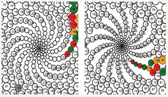
Figure 7: Patterns generated with COP = 0, V= 1 and COP = 0, v=1.375.

These patterns exhibit a degree of spiral structure but feature significant empty spaces between EPPs. Previous studies [30,35,39,45-47], have suggested that dense packing of primordia is a defining characteristic of spiral patterns. Based on this principle, it has been hypothesized that an additional mechanical force — external pressure directed toward the center plays a role in minimizing inter-EPP spacing during morphogenesis.

To conduct a statistical evaluation of the recursive biomechanical model, 644 patterns were generated by systematically varying two parameters:

• Growth rate parameter (v) ranging from 0.5 to 3.25, with increments of 0.125.
• Coefficient of outside pressure (COP) ranging from 0 to 1.4, with increments of 0.05.

Due to space constraints, the full set of 644 generated patterns is not included in this publication. However, researchers can independently generate patterns with various parameter settings by executing the biomodel_ statistic program (Appendix A). Additionally, Appendix C provides guidance on modifying the program to generate all 644 patterns in a single execution.

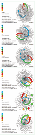
Figure 8: Sample Patterns Generated by biomodel_statistic program.

Figure 9 and Figure 10 summarize the analysis of over 600 patterns, with each pattern represented as a colored square at the intersection of specific v and COP values.

Figure 9: Distribution of generating recurring series.

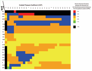
Figure 10: Relative Deviation between Theoretically Predicted and Computed Distances from the pattern’s center to EPP’s center.

Figure 9 employs a color-coded system to depict the distribution of generating recurrent sequences (parastichy indices), while Figure 10 visualizes the relative deviation between the theoretical and computed distances from the pattern center to each EPP.

Video 6. Execution of the biomechanical model over time. The outcomes of the biomodel_video program are demonstrated in Videos 6. The selected v and COP values for the three segments in Video 6 illustrate the model’s behavior across different parameter ranges:

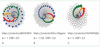
Video 6A https://youtu.be/qBZrIjCBfc0: parameters have low values. Both

Video 6B https://youtu.be/KAw_GUgqyno: Growth rate is low, while external pressure is high.

Video 6C https://youtu.be/54zP4dUtQQs: Both parameters have high values.

Figure 9 and Figure 10 reveal two distinct anomalous zones that coincide in both illustrations. The first is a horizontal region at v=0.5, where the generated patterns do not exhibit a spiral structure. This can be attributed to the fact that at v=0.5, all EPPs maintain the same diameter from the moment of their formation, as dictated by Formula 5. While this issue could potentially be addressed by modifying the model to include more complex functions— such as allowing the “newborn” EPP to grow only during its initial step—the authors have intentionally opted for the simplest possible mathematical functions. This approach ensures that the algorithm remains transparent, and the results are easily verifiable. The second anomalous zone appears as a vertical line at COP = 0, representing patterns that form in the absence of external pressure. Since these two extreme cases do not occur in real botanical structures, they remain theoretical constructs within the model.

All other patterns generated by the biomodel_statistic program with parameters v>0.625 and COP > 0 exhibit a relative deviation of less than 4% between the theoretically predicted and computed distances from the pattern’s center to each EPP (Figure 10). This finding serves as strong empirical validation of the biomechanical model’s reliability in explaining spiral phyllotaxis morphogenesis. A model based solely on Newtonian mechanics shows that the emergence of spiral patterns requires neither unknown forces nor information interactions between primordia.

Figure 9 shows that over 50% of the squares are marked in red, corresponding to Fibonacci phyllotaxis. The remaining patterns, in the region where v>0.625 and COP > 0, are associated with only four different generating recurrent sequences. Patterns with generating series {3,11} and {3,8} occur predominantly in regions with low COP values across the full range of growth rate parameters. These patterns are relatively rare in nature, suggesting that most plant species exhibit COP > 0.5.

Phyllotactic patterns corresponding to the Lucas generating sequence {1,3} [8], are the second most frequently observed in nature. As indicated in Figure 9, these patterns occupy the region where both v and COP attain their maximum values. This observation suggests a fundamental relationship between the generating sequence of a pattern and the interplay of v and COP. This insight is particularly significant, as no prior studies have offered a well-founded hypothesis explaining the differing morphogenetic pathways leading to Fibonacci and Lucas phyllotaxis.

Analysis of Video 6 and Figure 11 yields several notable findings.

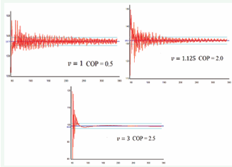
Figure 11: Evolution of the Divergence Angle.

The most important is that during the initial 100 iterations of the model, EPPs exhibit quasi-chaotic motion, with no apparent spiral structure. The divergence angle fluctuates widely. However, after approximately 100 iterations, the emergence of a well-defined spiral structure becomes evident in Video 6, with the divergence angle stabilizing within 2.5% of its theoretical value (Formula 2), as indicated by the cyan lines in Figure 11. Notably, as one progresses from Figure 11A to Figure 11C, the graph becomes progressively smoother. This trend is attributed to increasing external pressure, which enhances structural rigidity and reduces divergence angle deviations per iteration.

Video 6 also reveals two distinct secondary effects that differentiate the simulated patterns from the idealized model described in [2,3]:

• Pattern rotation;
• Pulsation of the overall pattern diameter.

The phenomenon of pulsation, characterized by periodic reductions in overall pattern diameter, arises from the fact that the angular distance between EPPs increases more rapidly than their diameters during growth. At a certain iteration, an EPP “falls” into an available space, causing a temporary contraction in the pattern’s overall size. A comparable phenomenon has been described by Hellwig [42], using centroidal Voronoi relaxation to model EPP displacement under external pressure. Fundamentally, this effect reflects the system’s tendency to evolve toward a minimal-energy configuration, favoring denser packing arrangements.

Pattern rotation is a direct consequence of the idealized assumptions inherent to the model. The EPPs are treated as incompressible, non-deformable discs with smooth surfaces, experiencing no frictional forces. In contrast, real primordia behave as elastic bodies capable of deformation without volume reduction, and their surfaces interact through frictional forces. Incorporating elasticity and friction into the model could potentially yield more biologically realistic pattern formations and a smoother distribution of generating sequences. However, as previously stated, the authors have deliberately employed the simplest possible mathematical framework to ensure that the model remains both computationally tractable and easily verifiable.

This study introduces a recursive biomechanical model to explain the morphogenesis of flat spiral phyllotaxis patterns based purely on classical mechanics. By simulating the interactions between growth pressure arising from the continuous expansion of phyllotactic elements and outside pressure, the model demonstrates how spiral structures emerge as a natural consequence of these forces. Computational implementation, which avoids any pre-programmed mechanisms to generate Fibonacci sequences or the golden angle, confirms that spiral phyllotaxis patterns can develop without invoking informational or unknown interactions between primordia.

Key findings include the emergence of Fibonacci and Lucas sequences as dominant patterns, with parameter areas where alternative phyllotactic patterns arise, such as those governed by less common generating series. The results also show that external pressure plays a crucial role in producing dense, biologically realistic patterns, distinguishing them from the loosely packed structures observed when this force is absent. Additionally, the stabilization of divergence angles and the reduction in structural irregularities over time reflect the system’s tendency toward an energy-minimizing configuration.

The model reveals two notable anomalous behaviors: the failure to form spiral structures at minimal growth rates and the generation of unrealistic patterns in the absence of external pressure. These insights offer a clearer understanding of how real-world biological systems operate within constrained parameter spaces. Moreover, the dynamic visualization of the pattern formation process uncovers secondary phenomena, such as pattern rotation and pulsation, which provide further evidence of the mechanical nature of phyllotaxis development.

Recently, a group of respected phyllotaxis researchers published a book “Do Plants Know Mathematics?” [41]. Of course, plants do not know mathematics, but they do obey the laws of physics.

We thank Arkadiy Boshoer (Brooklyn, NY) for the criticisms and assistance in preparing this article.

1. Rozin B. Towards solving the mystery of spiral phyllotaxis. Progress in Biophysics and Molecular Biology. 2023; 182: 8-14.
2. Rozin B. Double Helix of Phyllotaxis: Analysis of the Geometric Model of Plant Morphogenesis. Brown Walker Press. 2020.
3. Rozin B. Biomechanical Model of Morphogenesis of Spiral Phyllotaxis Patterns and its Computer’s Visualization. Am JBiomed Sci Res. 2024; 22.
4. Braun A. Vergleichende Untersuchung ü ber die Ordnung der Schuppen an den Tannenzapfen als Einleitung zur Untersuchung der Blattstellung ü berhaupt. Nova Acta Ph Med Acad Cesar Leop Carol Nat Curiosorum. 1831; 15: 195-402.
5. Schimper CF. Geometrische Anordnung der um eine Axe periferischen Blattgebilde. Verhandl. Schez. Naturf. Ges.1836; 21: 113-117.
6. Golé C, Dumais J, Douady S. Fibonacci or quasi-symmetric phyllotaxis. Part I: why? Acta Soc Bot Pol. 2016; 85: 3533.
7. Church AH. On the Interpretation of Phenomena of Phyllotaxis. New York: Hafner Pub. Co. 1920.
8. Jean R. Phyllotaxis: A Systemic Study in Plant Morphogenesis. Cambridge University Press. 1994.
9. Adler I, Barabe D, Jean RV. A History of the Study of Phyllotaxis. Ann Botany. 1997; 80: 231-244.
10. Barabe D, Lacroix C. Phyllotactic Patterns: A multidisciplinary approach. World Sci. 2020.
11. Rozin B. Three ways to confirm the correctness of the biomechanical model of the morphogenesis of spiral phyllotaxis. Genome Biol Mol Genet. 2024; 1: 010-014.
12. Turing AM. The Chemical Basis of Morphogenesis. Philosophical Transactions of the Royal Society of London. Series B, Biological Sciences. 1952. 237: 37-72.
13. Turing AM. Morphogen theory of phyllotaxis, in Morphogenesis. 1992; 3.
14. Hofmeister W. Allgemeine Morphologie der Gewachse, Handbuch der Physiologischen Botanik. Engelmann, Leipzig. 1868
15. Douady S, Couder Y. Phyllotaxis as a Dynamical Self Organizing Process Part I, II, III. J Theoretical Biol. 1996; 178: 255-312.
16. Hernandez LF, Palmer JH. Regeneration of the Sunflower Capitulum after Cylindrical Wounding of the Receptacle. Am J Botany. 1998; 79: 1253-1261.
17. Hertel R. The Mechanism of Auxin Transport as a Model for Auxin Action *. Zeitschrift für Pflanzenphysiologie. 1983; 112: 53-67.
18. Bainbridge K, Guyomarc’HS, Bayer E, Swarup R, Bennett M, Mandel T, et al. Auxin influx carriers stabilize phyllotactic patterning. Genes Dev. 2008; 22: 810-823.
19. Deb Y, Marti D, Frenz M, Kuhlemeier C, Reinhardt D. Phyllotaxis involves auxin drainage through leaf primordia. Development. 2015.
20. Godin C, Golé C, Douady S. Phyllotaxis as geometric canalization during plant development. Development. 2020; 147.
21. Reinhardt D. Regulation of phyllotaxis. Int J Dev Biol. 2005; 49.
22. Jönsson H, Heisler M, Shapiro B, Meyerowitz E, Mjolsness E. An auxin- driven polarized transport model for phyllotaxis. Proceedings of the National Academy of Sciences of the United States of America. 2006; 103: 1633-1638.
23. Sahlin P, Söderberg B, Jönsson H. Regulated transport as a mechanism for pattern generation: Capabilities for phyllotaxis and beyond. J Theor Biol. 2009; 258: 60-70.
24. Jiang Z, LIU D, WANG T, LIANG X, CUI Y, LIU Z, et al. Concentration difference of auxin involved in stem development in soybean. J Integrative Agriculture. 2020; 19: 953-964.
25. Yang L, Zhu M. The Interconnected Relationship between Auxin Concentration Gradient Changes in Chinese Fir Radial Stems and Dynamic Cambial Activity. Forests. 2022; 13: 1698.
26. Kuhlemeier C, Reinhardt D. Auxin and phyllotaxis. Trends Plant Sci. 2001; 6: 187-189.
27. Bravais L, Bravais A. Essai sur la disposition generate des feuilles. Ann Sci Nat Bot. 1839; 12: 5-14.
28. Mitchinson G. Phyllotaxis and the Fibonacci Series. Sci. 1977; 196: 270-275.
29. Niklas KJ. The Role of Phyllotactic Pattern as A “Developmental Constraint” On the Interception of Light by Leaf Surfaces. Evolution. 1988; 42: 1-16.
30. Niklas KJ. Plant Biomechanics. An Engineering Approach to Plant Form and Function. University of Chicago Press, Chicago. 1992.
31. Lee HW, Levitov L. Universality in Phyllotaxis: a Mechanical Theory. 2010.
32. Adler, I. A model of contact pressure in phyllotaxis. J Theor Biol. 1974; 45: 1-79.
33. Adler, I. A model of space filling in phyllotaxis. J Theor Biol. 1975; 53: 435-444.
34. Adler I. Solving the Riddle of Phyllotaxis: Why the Fibonacci Numbers and the Golden Ratio Occur on Plants. World Scientific. 2012.
35. Vogel H. A better way to construct the sunflower head. Math Biosci. 1979; 44: 179-189.
36. Roberts DW. A contact pressure model for semi-decussate and related phyllotaxis. J Theor Biol. 1977; 68: 583-597.
37. Roberts DW. A chemical contact pressure model for phyllotaxis. J Theor Biol.1984; 108: 481-490.
38. Roberts DW. The chemical contact pressure model for phyllotaxis— Application to phyllotaxis changes in seedlings and to anomalous phyllotaxis systems. J Theor Biol. 1987; 125: 141-161.
39. Ridley JN. Computer simulation of contact pressure in capitula. J Theor Biol. 1982; 95: 1-11.
40. Ridley JN. Ideal phyllotaxis on a general surface of revolution. Math Biosci. 1986; 79: 1-24.
41. Douady S, Dumais J, Golé C, Pick N. Do Plants Know Math? Unwinding the Story of Plant Spirals, from Leonardo da Vinci to Now. Princeton University Press. 2024.
42. Hellwig H, Engelmann R, Deussen O. Contact pressure models for spiral phyllotaxis and their computer simulation. J Theor Biol. 2006; 240: 489-500.
43. Richards FJ. The geometry of phyllotaxis and its origin. Symposium of the Society for Experimental Biology. 1948; 2: 217-245.
44. Richards FJ. Phyllotaxis: Its quantitative expression and relation to growth in the apex. Phil. Trans R Soc Lond. 1951; 235: 509-564.
45. Mughal A, Weaire D. Theory of cylindrical dense packings of disks. Phys Rev. 2014; 89: 042307
46. Mughal A. Weaire D. Phyllotaxis, disk packing, and Fibonacci numbers. Phys Rev. 2017; 95: 022401
47. Dixon R. The Mathematics and Computer Graphics of Spirals in Plants. Leonardo. 1983; 16: 86-90.
48. Lagarias JC, Mallows CL, Wilks AR. Beyond the Descartes Circle Theorem. The American Mathematical Monthly. 2002; 109: 338-361.