The purpose of this paper is to develop the fractional stochastic nonlinear differential equation approach (FBM) to apply this in the study of the evolution in time of infected number by coronavirus in countries where the number of infected is large. The rises and falls of epidemiologic weeks of novel cases are treated as fractional white noise BH (t); 1/2 < H < 1, in the model for spreading of epidemiologic week of novel cases. Since the FBM approach provide a useful model for a host of natural time series presented by scientists, engineers and statisticians, we apply this formalism to study the spreading of coronavirus. Moreover, we use the rescaled range analysis (RS) to determine the Hurst index of the time series of epidemiologic weeks of novel cases which exhibits a Hurst index much larger than 1/2, what means that the time series has a very distinct behavior from a random walk or that the nth value of time series up time t 0 is independent of all the values before, t < t 0 .

• Fractional Stochastic • Nonlinear Differential Equation • Hurst Index

Lima LS (2025) Fractional Stochastic Nonlinear Differential Equation Approach for Evolution in Time of Epidemiological Systems. JSM Math Stat 7(1): 1022.

It is well known that FBMs can be employed to model the spread of infectious diseases, including COVID-19 [1-10]. These fractional noises also known as fractional Brownian motions incorporate both fractional calculus and stochastic elements, allowing the inclusion of long- range dependence and random fluctuations in the modeling process. However, the use of fractional calculus in epidemiology is a relatively advanced and specialized approach. The basic form of a fractional stochastic differential equation can be written as: dX(t) = aX(t)dt + bX(t)dBH (t), where X(t) represents the state variable (e.g., the number of infected individuals), the a and b are constants representing the deterministic and stochastic components, respectively, dt is the differential time increment, dBH (t) is the fractional Wiener process, of fractional order H where H ∈(1/2, 1).

The mathematical modeling for spreading of diseases has been per- formed since long time ago, where the model was known be given by dN/dt = aN3 + bN2 -cN, being the parameters a and b into the range a > 0 and 0 < a < b. Taking some randomness in these parameters, we get a more realistic model to treat real situations [11-16]. The purpose of this paper is to model the novel cases of epidemiologic weeks using the fractional white noise calculus approach. We analyze the rises and falls of novel cases of coronavirus reported by the public healthy agencies in countries as Brazil and India where the low number tests performed in the populations leads to a large uncertainty in the official data. Due to possibility that the dynamics of novel cases must exhibit long-range correlations thus, it mays be described in terms of long-memory processes [17].

The use of the standard stochastic calculus has been many employed in the literature for the study of the time behavior of time series of stock prices [16,18-21]. Moreover, the use of the stochastic differential equations that corresponds to the case H = 1/2, was used recently for us to study the spreading of coronavirus in Ref. [4]. Besides, the modeling based in the fractional stochastic differential equation has been used in [3,5-7]. The stochastic dynamics smoking with a non-Gaussian noise was studied in Refs. [22-24]. The dynamics of a stochastic COVID- 19 epidemic model with jump-diffusion, was analyzed in [22]. The stochastic susceptible-infected-recovered (SIR) dynamics expressed using the Itˆo calculus has been pro- posed in Refs. [25-31]. The statistical analysis described by the master equation and transition rates for the infection process was made in Ref. [32]. The statistical inference in the epidemic model for the Ebola virus was per- formed in [33]. The discrete-time epidemic model with binomial distribution has been used to study the trans- mission rate of covid in [34].

A statistical model for the health care impact of COVID-19 in India has been studied in [35]. Moreover, the effect of immunization through vaccination on the susceptible–infected–susceptible (SIS) epidemic spreading model was analyzed in [36]. Here, we propose the analysis based on the fractional Brownian motion to study the dynamics of epidemiologic weeks of novel cases of coronavirus. The plan of this paper is the following. In section II, we describe the fractional white noise analysis as a model for spreading epidemiological systems. In section III, we present the numerical results and the long range memory analysis, using the rescaled range (RS) analysis. In the last section IV, we present our conclusions and final remarks.

The fractional Brownian motion (BMF) is defined as a family of Gaussian processes, being introduced by Kol- mogorov in [37], and indexed by the Hurst parameter H into the range 1/2 < H < 1. Being the first application made by Hurst in 1951 [38,39]. Such fractional Brownian motion was defined in Refs. [40, 41,42] where for each value of H, a real-valued Gaussian process BH (t), t ≤ 0 is defined by ⟨BH (t)⟩ = 0 and ⟨BH (t)BH (s)⟩ = the fractional Brownian motion is the standard Brownian motion or Wiener process. Moreover, we consider H restricted to range 1/2 < H < 1 and apply this as well as its modifier to model the infected number by coronavirus N (t) of epidemiologic weeks of novel cases. The model of spreading of novel cases N (t) is given by add of the least square fit g(t) to the logistic model with fractional noise which takes into account the isolation conditions and the vaccination of the population in each country, what has smoothing the curve of novel cases. Moreover, whether t → BH (t) is differentiable into the Schwartz space S(R) of rapidly decreasing smooth functions, being (SH )∗ His the dual of (S)H.

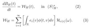
We have that the BH -integration theory of Eq. (1) is based on using of ordinary products path-wise and leads to an integral that for integrands g(t, ω) is defined where ?: a = t0 < t1 << tn = b is a partition of each interval [a, b] and ? = max0≤k≤n−1 (tk+1,tk ). These integrals do not have an expectation zero and are called fractional path-wise integrals. Here, we considerate the BH -integral considered in Ref. [43], defined by

Definition: Suppose g: R(S)∗ His a given function such that g(t) WH (t) is integrable in (S)∗ H. Then we definite the fractional stochastic integral of Itˆo type, by

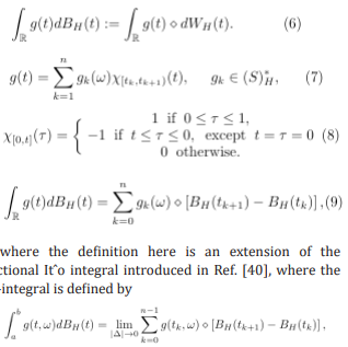
Where ? denotes the Wick’s product [40-47]. These integrals that use the Wick’s product are known as fractional Itˆo integrals with reference to corresponding situation of standard Brownian motion [41,42]. Due to the behavior of novel cases, we consider the deterministic part adjusting to the data of epidemiologic weeks of novel cases using a suave curve. The aim is simply provide a smoothed version of the time series using standard methods as the lowest regression. Furthermore, we aim to calculate the ensemble of all possible trajectories using the fractional behavior into the range of large t values reflects in an increase of the uncertainty in the official data and to the low-number of test performed in the populations. For modeling of the zigzag behavior of novel cases, we add a random noise term in the logistic model for spreading of infectious number as given by Eq. (1) in order to simulate the effect of rises and falls of novel cases [4]. We have that comes from the least squares Fit to the set of data into the period considered. The case a ? 0.017, b ? 0.26 and c ? 0.13 and without randomness (Γ = 0,) corresponds to the very known logistic model for the small- pox. Moreover, the daily fluctuations with a weekly cycle of reported cases have been observed in many countries and are due to the diagnostic and data reporting practices [48].

We write the BMF model that is a Gaussian pro- cess WH (t), t > 0 with zero mean and stationary in crements and variance given by W 2 (t) = t2H . The sample path of the BMF model is a fractal curve with fractal dimension d = 1/H, where H = 1/2 corresponds to the standard Brownian motion whose incre- ments ?WH (t) = WH (t + 1) WH (t) are statistically independent. For H = 1/2 the increments ?WH (t) are known as fractional white noise, showing long-range correlation as ⟨?WH (t + h)?WH (t)⟩ ? 2H(2H − 1)h2H−2, for h → ∞. For H ∈ (1/2, 1) the increments are positively correlated exhibiting thus a persistent behavior. For H ∈ (0, 1/2), the increments are negatively correlated, showing anti-persistence. For H = 1/2, we write the Wiener increment as dWH(t) ∼ where RG is an aleatory generator number with Gaussian distribution of mean zero and variance. In following, we write the Eq. (1) in the discrete form with the time step ?t used in the simulations as ?t = 0.1, with t running along chosen units (say seconds, minutes, days or weeks). In Figure 1, we present the simulation of the model Eq. (1 for a particular set of values of parameters a, b, c and Γ(N (t), t). In (a) we plot the epidemiologic week of novel cases reported in Brazil.

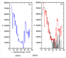
Figure 1 Simulation of the model Eq. (1 for the particular set of values of parameters a, b, c and Γ (N (t), t). (a) Data of epidemiologic week of novel cases reported in Brazil in 2023 year. (b) The time series of the model Eq. (1), for values of Hurst exponent: H = 1/2. The red-square line are the epidemiologic week of novel cases reported and the blackline is the result of the simulation of the model for set of parameters a = b = c = 0 and Γ = g

In plot (b), We plot the time series of model Eq. (1) for the value of Hurst parameter as H = 1/2. The red-square line are the data of epidemiologic week of novel cases reported and the black-line is the result of the simulation of the model for set of parameters a = b = c = 0 and Γ = g. In Figure 2, we perform simulations of the model Eq. (1 for H = 1/2 and Γ = g and different values of (a, b, c). (a) We plot the time series for the values of (a, b, c) such as (a, b, c) = (1.0, 2.0, 1.0) x10−10 (red-circle-line), (a, b, c) = (5.0, 10.0, 5.0) 10−10 (green-square-line), (a, b, c) = (5.0, 10.0, 5.0)x10−9 (blue-triangle-up-line). In plot (b) we present the behavior for values of pa- rameters a, b, c and for (a, b, c) = (0, 0, 0), that is represented as magenta-line: (a, b, c) = (1.0, 2.0, 1.0) x 10−10 (red-line), (a, b, c) = (5.0, 10.0, 5.0) x 10−10 (greenline), (a, b, c) = (5.0, 10.0, 5.0) x10−9 (blue-line). For a, b, c, we have that the drift term of the model above is given by a polynomial of third order in Nt . In general, a point N0 ∈ R in the model Eq. (1) is called a regular point if is locally integrable, L1loc(N0 ) and hence

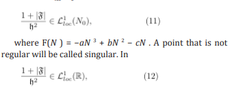
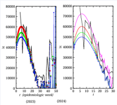
Figure 2 Simulation of the model Eq. (1 for H = 1/2 and Γ = g. (a) We plot the time series for different values of (a, b, c) parameters such as (a, b, c) = (1.0, 2.0, 1.0) × 10−10 (red-circle-line), (a, b, c) = (5.0, 10.0, 5.0) × 10−10 (green-square-line), (a, b, c) = (5.0, 10.0, 5.0) × 10−9 (blue-triangle- up-line)and H = 1/2. (b) Behavior for different values of pa- rameters a, b, c. (a, b, c) = (0, 0, 0) mangueta-line, (a, b, c) = (1.0, 2.0, 1.0) × 10−10 (red-line), (a, b, c) = (5.0, 10.0, 5.0) ×10−10 (green-line), (a, b, c) = (5.0, 10.0, 5.0)×10−9 (blue-line).

then there exist a unique solution for the model above, Eq. (1). The behavior of the solution at + and singularities is discussed in Ref. [49]. In Figure 3, we per- form simulations of the model Eq. (1). We plot the time series for different values of Hurst index H. We con- sider the set of parameters (a, b, c) such as (a, b, c) = (1.0, 2.0, 1.0) x10−10. We get that the model fits better when (a, b, c) = (1.0, 2.0, 1.0) x 10−10 and the value of the Hurt index is close to H = 1, that is in accordance with the value of the Hurst index obtained by rescaled range method H1 for the time series of epidemiologic weeks data.

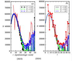
Figure 3 Simulation of the model Eq. (1) for different values of H and Γ = g. (a) We plot the time series for different values of Hurst index H. We consider the set of parameters (a, b, c) such as (a, b, c) = (1.0, 2.0, 1.0) × 10−10. The red-solid-line correspond to the data of epidemiologic weeks of novel cases reported in Brazil in (2023).

There are several estimators for the Hurst exponent such as rescaled range (RS) analysis, multifractal and detrended fluctuation analysis [50,51] that differ basically by the choice of the fluctuation measure. In Figure 4, we present the Log-Log graphic with objective to determine the Hurst index. We use the RS analysis, where the Hurst exponent is directly obtained and it is used as a measure of long-term memory of time series. It relates with the autocorrelations of the time series and the rate in which this decrease as the lag between pairs of values increases. The start point of the method is to determine the standard deviation using the mean field approach as and the range Rt of the series where H is the Hurst index. We get the value of the Hurst exponent using the RS method for time series of epidemiologic weeks of novel cases as H = 1.166(5). The numerical results display a Hurst index close to H = 1, being very far from the value for the standard Brownian motion H = 1/2. In spite of the constant value H ~1.17 obtained into the range considered, in a real situation, we must have a time dependent H = H(t) that is, the estimator is relevant into the current context and must be time dependent. The value found for the data set indicates thus, a strongly persistent behavior for the time series N (t) of epidemiologic week of novel cases reported.

In brief, we have analyzed the behavior of novel cases of epidemiologic weeks of coronavirus using the fractional white noise calculus, with the aim to model the rises and falls of these. We get that the model with H~1 fits better to the set of data reported. This value is closer to the value obtained for the time series using the RS method. The variability in the time series for instance is mostly due to the case numbers reports not being filled on weekends, leading to a large-amplitude oscillation in the data. Moreover, due to the large uncertainty in the official case numbers reported which is a consequence of the low number of tests performed in the population and to underreporting, we have a large uncertainly in the results divulged what becomes necessary the addition of random terms in the equations that model the time evolution of infected numbers.

We get a Hurst index close to H~1.17 for the time series of epidemiological weeks indicating so, a large deviation from the result H = ½ which corresponds to the standard stochastic calculus. An additional analysis whether fractional Gaussian noise is the best phenomenological approach to the fluctuations of coronavirus data can be made in a future work. The starting point could be to implement schemes as detrended fluctuation analysis, with possible free parameters, and a larger database that is, coronavirus data from many countries. Nevertheless, we must be careful in using of BMF and Gaussian noise with algebraic correlations for further investigation of data-driven what correlation structure the fluctuations display across different data sets.

1. Giordano G, Blanchini F, Bruno R, Colaneri P, Di Filippo A, Di Matteo A, et al. Modelling the COVID-19 epidemic and implementation of population- wide interventions in Italy. Nat Med. 2020; 26: 855.
2. Gatto M, Bertuzzo E, Maria L, Miccolid S, Carraroe L, Casagrandia R, et al. Spread and dynamics of the COVID-19 epidemic in Italy: Effects of emergency containment measures. PNAS. 2020; 117: 10484.
3. Lima L. Fractional Brownian motion analysis for epidemic spreadingof diseases. 2021.
4. Lima LS. Dynamics based on analysis of public data for spreading of disease. Sci Rep. 2021; 11: 12177.
5. Atangan A, Araz SI. Fractional Stochastic Differential Equations Applications to Covid-19 Modeling, Industrial and Applied Mathematics (INAMA). Springer Singapore. 2022.
6. Lima LS. Fractional Stochastic Differential Equation Approach for Spreading of Diseases. Entropy. 2022; 24: 719.
7. Omar OAM, Elbarkouky RA, Ahmed HM. Fractional stochastic models for COVID-19: Case study of Egypt. Results in Phys. 2021; 23: 104018.
8. Fanelli D, Piazza F. Analysis and forecast of COVID- 19 spreading in China, Italy and France. Chaos Solitons Fractals. 2020; 134: 109761.
9. Boccaletti S, Ditto W, Mindin G, Antangana A. Modeling and forecasting of epidemic spreading: The case of Covid-19 and beyond, Chaos Solitons Fractals. 2020; 135: 109794.
10. Ndairou F, Area I, Nieto JJ, Torres DFM. Mathematical modeling of COVID-19 transmission dynamics with a case study of Wuhan. Chaos Solitons Fractals. 2020; 135: 109846.
11. Gardiner C. Stochastic Methods, A Handbook for the Natural and Social Sciences, Fourth edition, Springer, New Zealand. 2009.
12. Øksendal B. Stochastic Differential Equations An Introduction with Applications, sixth edition. Springer-Verlag, Oslo. 2003.
13. Applebaum D. L´evy Processes and Stochastic Calculus. Cambridge university press. 2009.
14. Richmond P, Mimkes J, Hutzler S. Econophysics and Physical Economics, Oxford. UK. 2013.
15. Jacobs K. Stochastic Processes for Physicists, Cambridge University Press. New York. 2013.
16. Steven E. Shreve, Stochastic Calculus for Finance II Continuous-Time Models, Springer. New York. 2004.
17. Vasconcelos GL. A Guided Walk Down Wall Street: An Introduction to Econophysics. Braz J Phys. 2004; 34: 1039-1065.
18. Lima LS, Oliveira SC. Two-dimensional stochastic dynamics as model for time evolution of the financial market, Chaos. Solitons & Fractals. 2020; 136: 109792.
19. Lima LS, Miranda LLB. Price dynamics of the financial markets using the stochastic differential equation for a potential double well. Physica A. 2018; 490: 828-833.
20. Lima LS, Santos GKC. Stochastic Process with Multiplicative Structure For the Dynamic Behaviour of the Financial Market. Physica A. 2018; 512: 222-229.
21. Lima LS, Oliveira SC, Abeilice AF, Melgaco JHC. Breaks down of the modeling of the financial market with addition of non-linear terms in the Itˆo stochastic process. Physica A. 2019; 526: 120932.
22. Almaz T, Saeed T, Zeb A, Tesfay D, Khalaf A, Brannan J. Dynamical analysis of stochastic COVID-19 epidemic model with jump-diffusion. Adv Differ Equ. 2021; 2021: 228.
23. Zeb A, Kumar S, Tesfay A, Kumar A. A stability analysis on a smoking model with stochastic perturbation. Int J of Numerical Meth for Heat & Fluid Flow. 2021.
24. Alzahrani A, Zeb A. Detectable sensation of a stochastic smoking model. Open Mathematics. 2020; 18: 1045-1055.
25. Simha A, Prasad RV, Narayana S. A simple Stochastic SIR model for COVID 19 Infection Dynamics for Karnataka: Learning from Europe. 2020.
26. Khan F, Ali S, Saeed A, Kumar R, Khan AW. Forecasting daily new infections, deaths and recovery cases due to COVID-19 in Pakistan by using Bayesian Dynamic Linear Models. PLoS ONE. 2021; 16: e0253367.
27. Mahrouf M, Boukhouima A, Zine H, Lotfi EM, Torres DM, YousfN. Modeling and Forecasting of COVID-19 Spreading by Delayed Stochastic Differential Equations. Axioms. 2021; 10: 18.
28. El Kharrazi Z, Saoud S. Simulation of COVID-19 epidemic spread using Stochastic Differential Equations with Jump diffusion for SIR Model, 7th International Conference on Optimization and Applications. ICOA. 2021.
29. Kareem AM, Al-Azzawi SN. A Stochastic Differential Equations Model for Internal COVID-19 Dynamics. J Phys Conf Ser. 2021; 1818: 012121.
30. Zhang Z, Zeb A, Hussain S, Alzahrani E. Dynamics of COVID-19 mathematical model with stochastic perturbation. Adv Differ Equ. 2020; 2020: 451.
31. Tesfay A, Saeed T, Zeb A, Tesfay D, Khalaf A, Brannan J. Dynamics of a stochastic COVID-19 epidemic model with jump-diffusion. Adv Differ Equ. 2021; 2021: 228.
32. Tome T, de Oliveira MJ. Stochastic approach to epidemic spreading. Braz J Phys. 2020; 50: 832.
33. Lekone PE, Finkensta BF. Statistical inference in a stochastic epidemic SEIR model with control intervention: Ebola as a case study. Biometrics. 2006; 62: 1170.
34. He S, yi Tang S, Rong L. A discrete stochastic model of the COVID-19 outbreak: Forecast and control. Math Biosci and Eng. 2020; 17: 2792.
35. Chatterjee K, Chatterjee K, Kumar A, Shankar S. Healthcare impact of COVID-19 epidemic in India: A stochastic mathematical model. Med J Armed Forces India. 2020; 76: 147.
36. Tom´e T, Silva ATC, de Oliveira MJ. Effect of immunization through vaccination on the SIS epidemic spreading model. Braz J Phys. 2021; 51: 1853.
37. Kolmogorov N. Kolmogorov equation and large-time behaviour for fractional Brownian motion driven linear SDE’s. Acad. URSS (N.S.). 1940; 26: 115.
38. Hurst HE. Long-Term Storage Capacity in Reservoirs. Trans Amer Soc Civil Eng. 1951; 116: 400.
39. Hurst HE. Methods of using long-term storage in reservoirs. Proc Inst Civil Engineers. 1956; 5: 519.
40. Ness V, Mandelbrot BB. Fractional Brownian motions, fractionalnoises and applications. SIAM Review. 1968; 10: 422.
41. Hu Y, Øksendal B. Infinite Dimensional Analysis, Quantum Probability and Related Topics. 2003; 6: 1.
42. Duncan TE, Hu Y, Pasik-Duncan B. Stochastic calculus for fractional Brownian motion I. Theory. J Control Optim. 2000; 38: 582.
43. Hu Y, Øksendal B, Sulem A. Stochastic Analysis and Related Topics. 1996; 5: 203.
44. Decreusefond L, Ustunel AS. Stochastic analysis of the fractional Brownian motion. Potential Anal. 1999; 10: 177-214.
45. Elliott RJ, Van der Hoek J. A general fractional white noise theory and applications to finance. Math Finance. 2003; 13: 301-330.
46. Gripenberg G, Norros I. On the prediction of fractional Brownianmotion. J Appl Probab. 1996; 33: 400-410.
47. Hu Y, Øksendal B, Sulem A. Optimal portfolio in a fractional Black– Scholes market. Mathematical Physics and Stochastic Analysis. 2000: 267-279.
48. Bergman A, Sella Y, Agre P, Casadevall A. Oscillations in U.S. COVID-19 Incidence and Mortality Data Reflect Diagnostic and Reporting Factors. Clini Sci Epidemiol. 2020; 5: e00544-20.
49. Cherny AS, Engelbert HJ. Singular Stochastic Differential Equations. 2004: 1858.
50. Gu GF, Zhou WX. Detrending moving average algorithm for multifractals. Phys Rev. 2010; E 82: 011136.
51. Shao YH, Gu GF, Jiang ZQ, Zhou WX, Sornette D. Comparing the performance of FA, DFA and DMA using different synthetic long- range correlated time series. Sci Rep. 2012; 2: 835.