In this note we present some numerical simulations of the asymptotic behaviour of a Harmonic Oscillator Differential Equation, within the framework of a recently defined generalized differential operator. To obtain these results, we have not proceeded as in the published results: varying the functions of the right-hand side of the system considered, but, on the contrary, in the differential operator used, the nuclei and the order used have been varied. In this way, a greater scope and generality are provided to the results obtained, which complement some known in the literature.

Nápoles Valdes JE, Ramirez BA, Moragues LS, Ferrini1 MA (2024) Numerical Simulation of Local Generalized Derivative for a Harmonic Oscillator. J Phys Appl and Mech 1(1): 1003.

In the last 60 years we have witnessed a remarkable development of a field of Physics-Mathematics, designated by the name of Non-Linear Mechanics. This term is probably not entirely correct, the changes have not occurred in Mechanics itself, but mainly in the techniques for solving its problems, especially those treated with the help of linear deferential equations, which now use non-linear deferential equations.

This is not a new idea in Mechanics. Indeed, these non-linear problems have been known since the studies of Euler, Poinsot, Lagrange and other geometers of that time, sufficient to illustrate this non-linear period of more than a century. The main difficulty of these studies, called classical, lies in the absence of a general method to treat these problems, which were treated mainly by special devices to obtain their solution. The LiØnard Equation

x′′ + f(x)x′ + g(x) = 0,                                                                   (1)

where f(x), g(x) are continuous functions f,g : R→R, f(x) > 0, xg(x) > 0,x ?= 0 and g(0) = 0, is a typical example of nonlinear deferential equations describing damped and forced oscillatory systems, see for example [1-13], and classical sources [14-16].

In this work, we are particularly interested in studying the forced-damped pendulum which is a non-homogeneous LiØnard equation whose expression is given by:

θ¨+ βθ? + sin(θ) = f cos(?t),                                                           (2)

where θ is the displacement angle, t is the time, β is the friction parameter, f is the magnitude of the external force and 

? is the frequency of the force. It should be clarified that for convenience the values of the local gravity acceleration, the mass of the particle and the length of the pendulum rod have been rescaled.

The pendulum equation is iconic in Physics and Mathematics for several fundamental reasons:

Application of Fundamental Principles: The pendulum equation, in its simplest form, describes the oscillatory motion of a pendulum under the action of gravity. It is a direct application of the principles of dynamics and the analysis of oscillatory systems, and provides a basis for understanding more complex phenomena.

Simplicity and Mathematical Elegance: In its linearized form (for small angles), the simple pendulum equation is an example of a second-order ordinary differential equation. Its solution reveals simple harmonic motion, which is fundamental in the study of oscillatory systems and waves. This simplicity and elegance in the solution make the equation a cornerstone in the study of physics and mathematics.

Importance in Oscillatory Systems: The analysis of the simple pendulum helps to understand the behaviour of many other oscillatory systems, from springs to electrical circuits. It is a specific case of a more general oscillation system and serves as a basic model for understanding more complicated phenomena.

Connections to Classical Physics and Mathematics: The pendulum equation connects to several fundamental concepts in classical physics, such as conservation of energy and equations of 

motion. Mathematically, it relates to the study of trigonometric functions and deferential equations.

Practical and Experimental Applications: The simple pendulum also has practical applications, such as in pendulum clocks, which were essential to the development of accurate timekeeping in the past. The study of the pendulum provides a way to understand gravity and time in a practical way.

In short, the pendulum equation is iconic because it encapsulates fundamental concepts of physics and mathematics in an accessible and elegant way, serving as a model and tool for a wide variety of studies in both disciplines.

The aim of this work is to analyse the phase diagrams of the system under fractional derivatives with different kernels studied in previous works [17], comparing with the known results of the current system. This comparison allows us to know the effect of each kernel on the system, and to estimate if any of them could be generalized to represent some physical effect.

Despite his predecessors, Galileo is the rst scientist associated with the experimental and theoretical study of the pendulum. The story is well known - true or false - of his discovery in 1583 or 1584 of the isochronism of the oscillations of the pendulum, observing a lamp suspended in the cathedral of Pisa.

Galileo’s rst written document on the isochronism of the pendulum is a letter of 1602 to Guidobaldo del Monte: “You must forgive my insistence in my desire to convince you of the truth of the proposition that the movements in the same quadrant of a circle are made at the same time”. In his famous “Dialogue”, he wrote: “The same pendulum makes its oscillations with the same frequency, or with little difference, almost imperceptible, when these are made by a larger circumference or on a very small one”. This is, of course, a wrong approach or, on a positive note, we can consider it to be a very primitive manifestation of what is, possibly, the rst basic tool in nonlinear science: linearization.

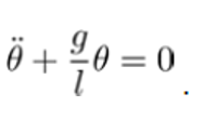
We know that isochronism is not a property of the solutions of the differential equation of the pendulum with length l:

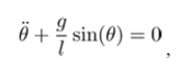
but in its linearized form:

Later contributions were made by Newton, Wendelin, Huggens, Euler, Poisson, Legrende, Jacobi, Georges Lemaitre and many more [18 20].

Phase plane analysis is a graphical method for studying the behaviour of solutions of dynamical systems. The basic idea of this method is to generate motion trajectories corresponding to various initial conditions and then examine the qualitative characteristics of the trajectories. In this way, information about the stability, periodicity or boundedness of the system can be obtained. In our case, we will keep the initial condition and vary, as we said before, the kernel and the order of the derivative, thus obtaining information about the effects of the fractional order derivative with nonlinearities and comparing the motion trajectories of a damped pendulum system between the fractional order derivative and its integer order counterpart. The numerical study of the pendulum has been treated using classical fractional derivatives and using the traditional phase plane approach: the initial conditions are varied, hence the difference in our approach and the results obtained [21 24].

The fractional calculus studies problems with derivatives and integrals of real or complex order, no necessary integer. As a purely mathematical field, the theory of fractional calculus was brought up for the rst time in the XVIIth century and since then many renowned scientists worked on this topic, among them Euler, Laplace, Fourier, Abel, Liouville and Riemann see [25]. Today there is a vast literature on this subject, many works and researchers multiply day by day in the world showing the most varied applications. The most common applications are currently found in Rheology, Quantum Biology, Electrochemistry, Dispersion Theory, Diffusion, Transport Theory, Probability and Statistics, Potential Theory, Elasticity, Viscosity, Automatic Control Theory,

Within this mathematical discipline there is a field called Local Fractional Calculus, which is very recent and has many applications (consult [26]). Although local operators have been used since the late 1950s, it was not until 2014 that a complete formalization was achieved, with the conformable derivative of [27]. Later, in 2018, we de ned a new type of di erential operator: non-conformable see [28,29] that has proven its usefulness in various applications. Both derivatives and other known ones were generalized in [30] see also [31,32] and it will be the operator that we will use in this work.

On the other hand, the fractional derivatives have been widely used to analyzed di erent physics systems which can exhibit chaotic behavior such as the ones described by Lienard’s equation (1). For this purpose, we use the definition of fractional derivative given by [30]

Definition 1 Given a function f: [0,+∞) →R. Then the N-derivative of f of order α is defined by

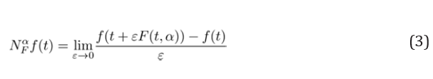
for all t > 0, α ∈ (0,1) being F(α,t) is some function. If f is α− differentiable in some (0,α), and , exists, then define 

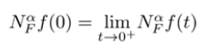
 note that if f is differentiable, then

 

where f′(t) is the ordinary derivative. The kernels we study are

F(t,α) = exp(t(1 − α)) F(t,α) = tα                                                   (4)

F(t,α) = t−α

F(t,α) = exp(t−α),

for orders 0.25, 0.5 and 0.75.

Numerical study of the pendulum equation is crucial for several reasons:

Accuracy in Nonlinear Behaviour: The simple pendulum equation is based on the assumption that the angle is small, allowing for a linear approximation. However, for large angles, the pendulum behaviour becomes nonlinear and more complex. Numerical methods allow analysing and predicting the pendulum behaviour in these nonlinear cases.

Simulation of Complex Systems: For coupled pendulums or more complicated pendulum systems, the equations become much more intricate and di cult to solve analytically. Numerical methods allow simulating and studying these complex systems to understand their dynamics and motion patterns.

Stability Analysis: Numerical methods help analyse the stability of solutions and the long-term behaviour of the system. This is essential in practical applications and in the design of systems that use pendulums, such as clocks or measuring devices.

Development of New Technologies: In engineering and applied physics, numerical analysis of pendulum systems can lead to the development of new technologies and devices. For example, in sensor design or oscillation and vibration research, numerical study provides detailed understanding that can improve performance and accuracy.

Education and Understanding: From an educational standpoint, numerical studies help students understand how mathematical models relate to the real world. Seeing numerical results and simulations in action can provide a clearer intuition about how the pendulum works under various conditions.

In summary, numerical study of the pendulum equation not only allows for a deeper understanding of pendulum behaviour under non-ideal conditions, but also has important practical applications in engineering, physics, and other related areas.

In order to determine the evolution of the system by numerical methods, equation (2) is expressed in a coupled system of three rst-order differential equations of the form

ω? = −βω − sin(θ) + f cos(?)

θ? = ω                                                                                           (5)

?? = ?

The problem of the global existence of solutions of the system (5), that is, the boundedness of the solutions at all future times, has been studied in [9,33] so our numerical study is justified. Using the formalism of fractional derivative and Definition 1, we obtain

ω? = F−1(t,α)(−βω − sin(θ) + f cos(?))

θ? = F−1(t,α)ω                                                                    (6)

?? = F−1(t,α)?

I                                       (7)

n order to solve equation (6) numerically, we use the time independent Runge-Kuta fourth-order method for ordinary differential equation (7). where yi+1 = (ωi,θi,?i) and g(yi,F−1(t,α)) represent the equation (6), such that

yi+1 = yi + (k1 + 2k2 + 2k3 + k4)/6.                                               (8)

In this particular simulation we worked with a h = 0.001, that is to say, a weighted precision of h4 = 10−12.

First, the results we obtain using ordinary derivatives are as follows

Why is the ordinary case included?

Why is the ordinary case included? First, because in Definition 1 if F ≡ 1 we obtain the ordinary derivative, i.e. it is a particular case of the generalized Pendulum Equation that we are studying and second, because the known numerical studies with fractional operators, compare their results with the ordinary case. This gives us a much more objective evaluation pattern [21,24].

At the following, the same cases are analysed for the different kernels mentioned before.

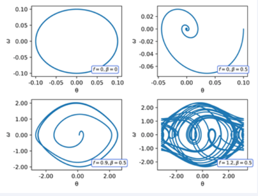
Figure 1 Phase diagram of the Pendulum of four cases: simple pendulum (f = 0,β = 0), damped pendulum (f = 0,β = 0.5, forced-damped pendulum in a limit cycle (f = 0.9,β = 0.5), and forceddamped pendulum in a chaotic regime (f = 1.2,β = 0.5).

Next, in (Figures 2-4), we show the asymptotic behaviour of (5), by means of the phase diagram using the kernel F(t,α) = tα, for α = 0.25, 0.5, 0.75. In this case, we are in the presence of a non- conformable derivative.

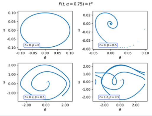
Figure 2 Phase diagram of the Pendulum with F(t,α = 0,75) = tα.

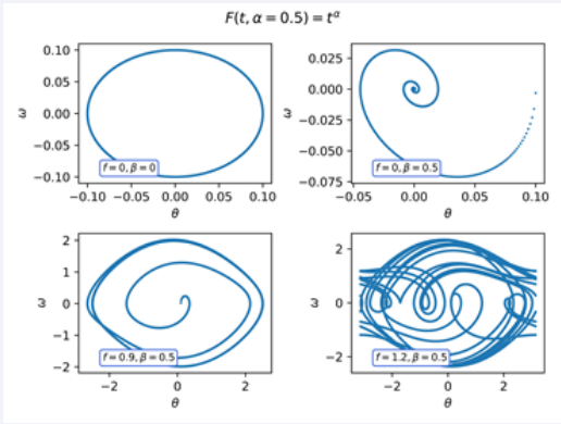
Figure 3 Phase diagram of the Pendulum with F(t,α = 0,5) = tα

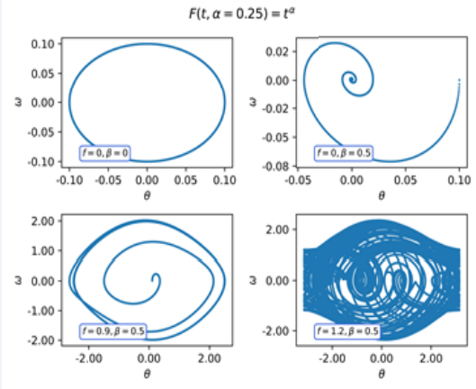
Figure 4 Phase diagram of the Pendulum with F(t,α = 0,25) = tα.

The qualitative behaviour of the system does not seem to change for any of the regimes. In this case, despite the relation tαω′(t) the kernel does not in uence the asymptotic behaviour of the solutions, under the parameters considered.

In (Figures 5-7), we show the phase diagram using the kernel F(t,α) = t−α, for α = 0.25, 0.5, 0.75. As in the rst case, the qualitative behaviour of the system does not seem to change for any of the regimes. However, in the (Figures 5) we observe that the pendulum simple regime appears to have energy dissipation.

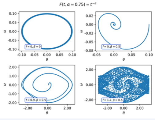
Figure 5 Phase diagram of the Pendulum with F(t,α = 0,75) = t−α

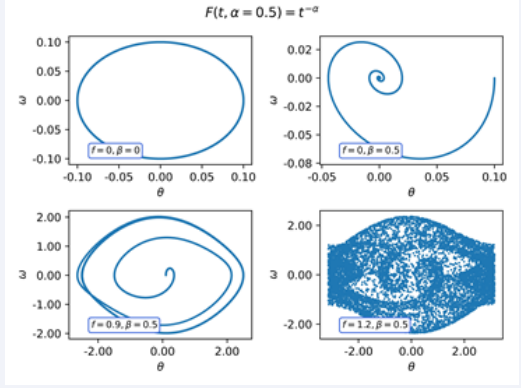
Figure 6 Phase diagram of the Pendulumr with F(t,α = 0,5) = t−α

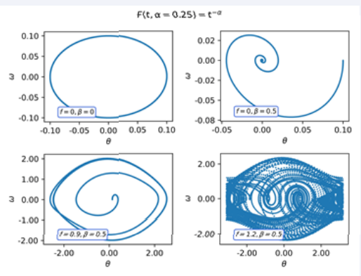
Figure 7 Phase diagram of the Pendulum with F(t,α = 0,25) = t−α

The observation we made in the previous case remains valid in this case. Next, in (Figures 8-10) we show the phase diagram from with F(t,α) = et−α, for α = 0.25, 0.5, 0.75. This operator local is a non- conformable derivative, let us note that this kernel, when t → +∞ tends to 1, that is, this kernel does not in uence the asymptotic behaviour of the solutions.

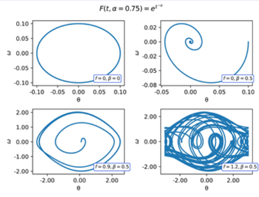
Figure 8 Phase diagram of the Pendulum with F(t,α) = et−α = 0,75.

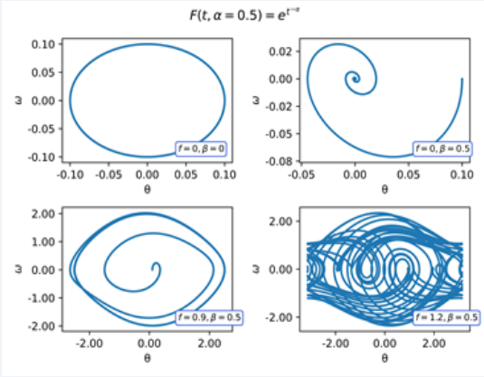
Figure 9 Phase diagram of the Pendulum with F(t,α) = et−α = 0,5.

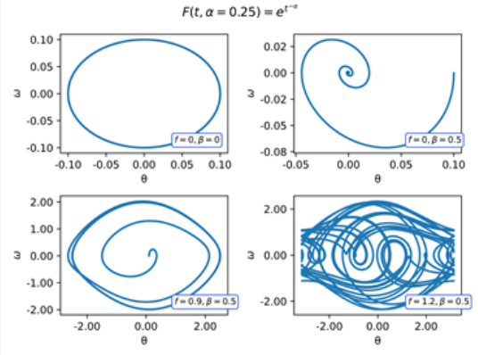
Figure 10 Phase diagram of the Pendulum with F(t,α) = et−α = 0,25.

In (Figures 14,15) we confirm this later by evolving the system to higher tempos, and observing the decrease of the energy of the system, in spite of the fact that β = 0.

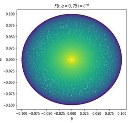
Figure 14 Phase diagram of the Pendulum in Simple regime with F(t,α = 0,75) = t−α up to a time of 5000.

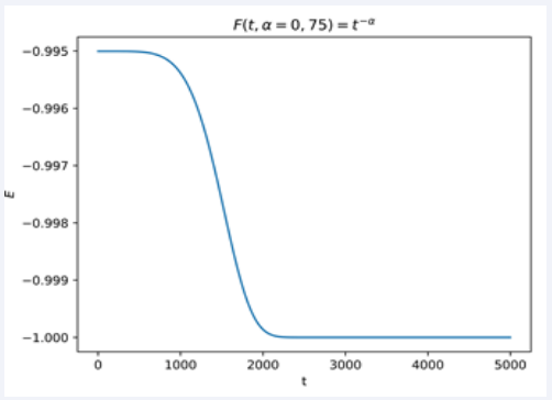
Figure 15 Energy versus time of the Pendulum with F(t,α = 0,75) = t−α up to a time of 5000.

In (Figures 11-13) we show the phase diagram using the conformable kernel F(t,α) = et(1−α), for α = 0.25, 0.5, 0.75, we observe that the evolution of the system is rapidly decelerating, soon reaching a stable point. Mathematically, this is due to the exponential growth as a function of time of the kernel used.

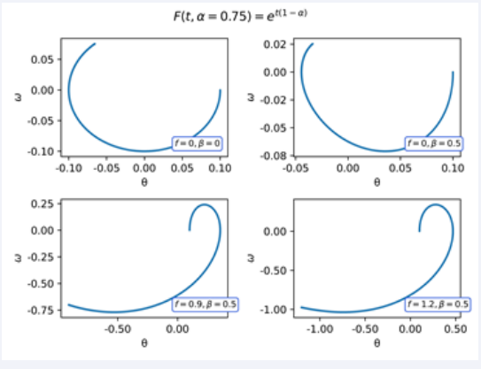
Figure 11 Phase diagram of the Pendulum with F(t,α) = et(1−α) = 0,75.

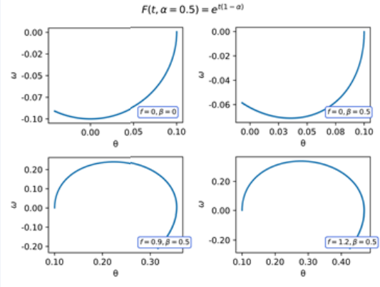
Figure 12 Phase diagram of the Pendulum with F(t,α) = et(1−α) = 0,5.

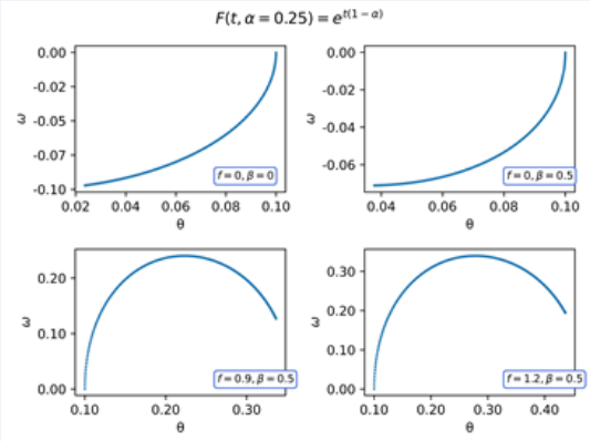
Figure 13 Phase diagram of the Pendulum with F(t,α) = et(1−α) = 0,25.

We know that a high gradient means that from one point to another nearby point the magnitude can present important variations (here a high or large gradient is understood as one whose magnitude is large). A small or null gradient of a magnitude implies that said magnitude hardly varies from one point to another. In the following picture the colour gradient indicates the time of each point, such that the time is longer as the color is brighter.

Let’s look at the following graph.

The high dissipation of energy in this case means that we are in the presence of a system with low complexity. The degree of complexity of a system indicates the evolutionary level of a system, that is, its thermodynamic status: how far it is from equilibrium and, in other words, how much entropy it produces to survive. By defining complexity as the measure of the distance from the state of thermodynamic equilibrium, which is the definitive state for all, we are postulating provisional states (temporary and local) that will be the object of study in the light of the complexity paradigm and that, therefore, go beyond the scope of this work.

In this work we have presented a set of asymptotic behaviours of the (5) using different kernels and with different orders, from these examples, we can obtain the following conclusion:

The study of the qualitative behaviour of the solutions, using conformable and non-conformable kernels, has provided the following regularity, it is not the type of kernel itself that is transcendental, but the behaviour at infinity of said kernel. For kernels with exponential growth to infinity, we conjecture that the phase portraits are altered, instead for behaviours at infinity of a similar order to t like tα, or when they tend to zero like t−α or when they tend to another constant like et−α the qualitative behaviours of the classical system are preserved.

We have obtained behaviours similar to the ordinary case, different from those reported in [21,24] obtained with classical fractional operators, defend in terms of integrals. It is clear that our results are closer to the classical results because we use local operators. This can better illustrate the study of other cases.

In this paper, using the Pendulum Equation as a basis, we have presented a set of numerical results that illustrate an idea inherent in research in applied sciences [34].

When using any mathematical model, the problem of the validity of the application of mathematical results to objective reality arises. If the result is highly sensitive to a small modification of the model, then even small variations of the model will lead to a model with different properties. Such results cannot be extended to the real process under investigation, because in the construction of the model a certain idealization is always carried out and the parameters are determined only approximately.

Moreover, in tasks related to practical problems, it is not enough, for example, to know that the solution exists. The non-mathematician can do little with an abstract theorem of existence. The mathematician, seeking a way out of this situation, provides procedures to “construct” the solution and since it is not always possible to nd quadrature, he tends to present procedures that involve an infinite collection of operations. Thus, if on the one hand, following the impulses of the internal logic of the development of mathematics, purely theoretical results on the solubility of equations grow in quantity and variety, on the other hand we have the following:

What does an exact solution mean to the experimental physicist?

How can this notion be interpreted, if it is known that the initial data are inexact?

As such, the mathematical model is never identical to the object under consideration, and the accuracy and reliability of the results is one of the most delicate problems in the application of mathematics. At this point, two cases must be distinguished: when the laws that determine the “behaviour” of the entity are well known and when our knowledge of said entity is insufficient. In the rst case, it is possible, a priori, to provide “limits” on the accuracy of the results; such it as an example to launch the automatic station Luna-1 (January 2, 1959) that opened the era of interplanetary lights, whose trajectory was obtained by means of a mathematical model where the known laws of mechanics intervened; the universality of these laws was the guarantee of application of the model to the cosmic apparatus created by man; in the second case, when constructing the mathematical model, it is necessary to make additional assumptions that have the character of hypotheses. The deductions obtained as a result of the investigation of such a “hypothetical model” have a conventional character in relation to the physical entity being studied.

Based on the above, it is then necessary to formulate a work strategy, where it is necessary to consider, for example, aspects such as the following:

1. Study the existence and uniqueness of the solutions.
2. Elaboration of algorithms (systems of pre-established rules depending on the nature of the process).
3. Analysis of the continuous dependence of the solution on the initial data.
4. Estimation of the algorithm errors and calculation errors.

However, in this case new problems arise, which we have already alluded to and which we will not repeat here, only to say that the resolution of a practical problem by a mathematician for a nonmathematician involves conclusions in which the mathematician and the specialist who works with him must necessarily intervene. In addition to all the above, we think that this work can serve as a guide and reference for other more complete works and that it has certain methodological advantages, namely that in other fields not considered, conclusions such as those provided here can be obtained.

• it allows conjectures to be made about general cases and, in certain cases where a false conjecture is made, to verify said falsehood,
• it usually considers, when faced with certain problems, simpler cases, the genesis of the problem, which can help greatly in the resolution of more complex problems.

As an illustration of this theory, we will present the “Loss of Equilibrium Stability and Selfoscillating Mode of Behaviour” for plane system. The loss of stability of an equilibrium state due to a change in parameters does not necessarily have to be associated with the bifurcation of the equilibrium state: stability can be lost not only by adjoining another state, but also by the same state.

Let us analyse the following reorganisations of the phase portrait of a planar system: √

1. By a change in the parameter the equilibrium state gives rise to a limit cycle (of radius ?, where the parameter di ers from the bifurcation value by ?). The stability of the equilibrium is transferred to the cycle and the equilibrium point is unstable.
2. A limit cycle collapses in the equilibrium state: the attractive domain of the equilibrium state disappears with the cycle and when the cycle disappears, it transfers its instability to the equilibrium state.

If our equilibrium state is the established behaviour of a real system, then under changes of parameters the following phenomena are observed in cases a) and b).

          i. After the loss of equilibrium stability a periodic oscillatory behaviour is established, the amplitude of the oscillations is proportional to the square root of the “criticality” (the difference between the parameter and the critical value, at which the equilibrium loses stability).

This form of stability loss is called “soft”, since the oscillatory behaviour, for a small value of criticality, di ers little from the equilibrium state.

        ii.  Before the state of stability loss is established, the domain of attraction of the state tends to be very small and when disturbances occur, the  domain of attraction disappears completely.

This form is called “hard”. Here the system leaves its stationary state with a jump to a different state of motion. This state can be another stable stationary state or some more complicated motion.

For an experimental physicist or an applied mathematician, these behaviours can be revealed with a numerical analysis such as the one we have presented, since in classical studies the parameters of the equation are the ones that vary, but this information is insufficient; with the incorporation of new differential operators that depend on both the order and the kernel, the panorama presented to the researcher is much more comprehensive.

Acknowledgment The authors would like to thank the reviewers and the Editor for their helpful comments and feedback, which made it possible to improve the quality of the work.

1. Chatzarakis GE, Nápoles Valdés, JE. Continuability of liønard’s type system with generalized local derivative. Discontinuity, Nonlinearity, and Complexity. 2023; 12: 1-11.
2. Fleitas A, Méndez JA, Nápoles JE, Sigarreta JM. On the some classical systems of Liénard in general context. Revista Mexicana de F sica. 2019; 65: 618-625.
3. Guzmán PM, Bittencurt LMLM, Nápoles Valdés, JE.. A note on stability of certain liénard fractional equation. International Journal of Mathematics and Computer Science. 2019; 14: 301-315.
4. Hale K, Hara T, Yoneyama T, Sugie J. Necessary and sufficient conditions for the continuability of solutions of the system x’=y-F(x), y’=-g(x). Applicable Analysis: An International Journal. 1985; 19: 169-180.
5. Hasan YQ, Zhu LM. The bounded solutions of LiØnard equation. Journal of Applied Sciences. 2007; 7: 1239-1240.
6. Helms LL. Introduction to potential theory. New York: Wiley- Interscience. 1969.
7. LaSalle JP. Some extensions of Liapunov’s second method. IRE Transaction on Circuit Theory. 1960; 7: 520-527.
8. Lugo LM, Nápoles V., JE,, Noya SI. On the construction of regions of stability. Pure and Applied Mathematics Journal. 2014; 3: 87-91.
9. Juan E. Nápoles Valdes. A continuation result for a bidimensional system of differential equations. Revista Integraci n. 1995; 13: 49-54
10. Juan E. Nápoles Valdes. On the global stability of non-autonomous systems. Revista Colombiana de MatemÆticas. 1999; 33: 1-8.
11. Juan E. Nápoles Valdes. On the boundedness and asymptotic stability in the whole of Liénard equation with restoring term. Revista de la Unión Matemática Argentina. 2000; 41: 47-59.
12. Juan E. Nápoles Valdes, Repilado RJA. On the boundedness and stability in global sense of the solutions of a two-dimensional system of differential equations. Revista Ciencias MatemÆticas. 1997; XVI: 71-74.
13. Lequn Peng, Lihong Huang. On global asymptotic stability of the zero solution of a generalized Lienard’s system. Applied Mathematics-a Journal of Chinese. 1994; 9: 359-363.
14. Liénard A. Etude des oscillations entretenues, Revue générale de l’électricité.. 1928; 23: 901-912, 946-954.
15. Van der Pol B. On oscillation hysteresis in a triode generator with two degrees of freedom. Phil. Mag. 1922; 43: 700-719.
16. Van der Pol B. On ‘relaxation-oscillations’. Philosophical Magazine. 1926; 2: 978-992.
17. Nápoles Valdés, Roa PM. Numerical simulations in a generalized Liénard’s type system. Ann Math Phys. 2023; 6: 187-195.
18. Juan E. Nápoles Valdés, C. Negrón Segura. From analytical mechanics to ordinary differential equations. 1994; 17: 190-206.
19. Juan E. Nápoles Valdes. The historical legacy of ordinary differential equations. (Self-)critical considerations. Boletín de Matemáticas. 1996; 1998: 53-79.
20. Juan E. Nápoles Valdes. A century of qualitative theory of differential equations. Revista Lecturas Matemáticas. 2004; 25: 59-111.
21. Baleanu D, Asad JH, Jajarmi A. The fractional model of spring pendulum: New features within different kernels. Proceedings of the Romanian Academy, Series A. 2018; 19: 447-454.
22. Baleanu D, Jajarmi A, Defterli O, Wannan R, Sajjadi SS, Asad JH. Fractional investigation of time-dependent mass pendulum. Journal of Low Frequency Noise Vibration and Active Control. 2024; 43: 196- 207.
23. Goncalves LN, Fernandes J, Ferraz A, Silva AG, Sebastiao PJ. Physical pendulum model: Fractional di erential equation and memory e ects. Am J Phys. 2020; 88: 962-975.
24. N’Doye I, Kirati TML. Stability and trajectories analysis of a fractional generalization of simple pendulum dynamic equation. 18th European Control Conference (ECC). 2019.
25. Machado JT, Kiryakova V, Mainardi F. Recent history of fractional calculus. Communications in Nonlinear Science and Numerical Simulation. 2011; 16: 1140-1153.
26. Juan E. Nápoles Valdes. The non-integer local order calculus. Phys Astron Int J. 2023; 7:163-168.
27. Khalil R, Al Horani M, Yousef A, Sababheh M. A new definition of fractional derivative. Journal of Computational Applied Mathematics. 2014; 264: 65-70.
28. Guzmán PM, Langton G, Lugo LM, Medina J, NÆpoles ValdØs JE. A new de nition of a fractional derivative of local type. J Math Anal. 2018; 9: 88-98
29. Nápoles Valdés, JE, Guzmán PM, Lugo LM. Some new results on non- conformable fractional calculus. Advances in Dynamical Systems and Applications ISSN 0973-5321. 2018; 13: 167-175.
30. Nápoles JE, Guzmán PM, Lugo LM, Kashuri A. The local non conformable derivative and Mittag-Leffler function. Sigma J Eng & Nat Sci. 2020; 38: 1007-1017.
31. Fleitas A, Nápoles Valdés JE, Rodr guez JM, Sigarreta JM. Note on the generalized conformable derivative. Revista de la UMA. 2021; 62: 443-457.
32. Zhao D, Luo M. General conformable fractional derivative and its physical interpretation. Calcolo. 2017; 54: 903-917.
33. Juan E. Nápoles Valdés. On the continuability of solutions of bidimensional systems. Extracta Mathematicae. 1996; 11: 366-368.
34. Juan E. Nápoles Valdés. From Lagrange to Arnold. Methodological remarks on a history of ordinary differential equations. Universidad de Holgu n Cuba. 1996; 129 p. Edited by the Universidad Tecnol gica Nacional Publishing House, 2006