In standard cosmology, Einstein’s Field Equations (EFE) were established as rulers that describe the dynamic evolution of the Universe [1]. Considering the cosmological principle the metric (solution for the EFE) that best fits the description of this dynamic evolution is the FLRW [2-5].

Over the EE a so-called standard cosmological model (ΛCDM) was formulated. This model is the one that best fits observational data obtained from new scientific ventures, such as the Planck project a.e. among others. However, this model faces some difficulties in theoretical justification for some observational notes that have so far been unresolved. Among these difficulties is the search for a phenomenological justification for anisotropies in the CMB power spectrum. One of these anisotropies corresponds to the so-called SACHS- WOLFE EFFECT (SWE), subject of this work.

The SWE [6], arises from the gravitational redshift suffered by the CMB during the Last Scatering Surface (LSS) combined with the effect (blueshift) of time dilation due to some scalar disturbance in the metric also when LSS. This effect is not constant across the sky due to differences in matter and energy densities during LSS [7-11].

- CMB ANISOTROPIES -

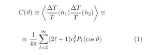
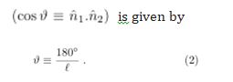
The correlation function (first definition) between two points, in a space with spherical symmetry, can be decomposed in the form (second definition)

where the relationship between ϑ and ? 

It is customary to adopt as Temperature fluctuations (y− axis) the function.

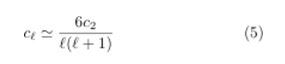
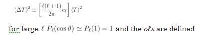 in terms of the observational data for large ?.

The monopole term (? = 0) is the constant isotropic mean temperature of the CMB ⟨T ⟩ = 2.7255 ± 0, 0006K with one standard deviation confidence. This term must be measured with absolute temperature devices such as the FIRAS instrument on the COBE satellite.

The CMB dipole represents the largest anisotropy which is in the first spherical harmonic (? = 1) a cosine function.

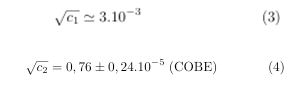
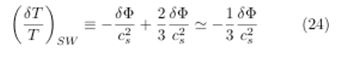
For small ones ?s [12],

It is customary not to represent these first two terms in the CMB power spectrum.

The SW and ISW occur on large scales (small ?s).

It is expected that there will be a peak in temperature variation in the photon radiation (from the CMB) in the LSS region due to the difference in pressure before and after the last scattering [13-19].

the physical dimension of the causal horizon in the LSS was worth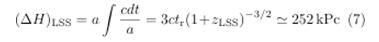 

However, the horizon that really matters is associated with the distance traveled by sound: the behavior of pressure oscillations It is known that the speed of sound at that time was

From the expression that converts distance into horizon angle in the spatially flat Universe model where h is the Planck constant 

To this ϑ corresponds  : approximate position of the first acoustic peak of Figure 1.

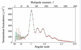
Figure 1 Power Spectrum (PS) of the Cosmic Microwave Background (CMB).

Consider the scalarly perturbed flat FLRW metric (conformal Newtonian gauge) in the form 

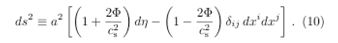
In this context, Φ corresponds to the Newtonian potential itself.

The Gravitational “Redshift”

Establishing the velocity of the fluid by  the Euler equation for a fluid with Total (T) internal energy ρ(T) becomes [11-24].

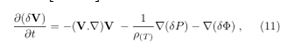
where corresponds to the action of some external force δF. If the only external force acting on the system is gravitational, we can identify the Φ of gravity with that of gravitational (10). Establishing , as each degree of freedom has associated with it the amount of energy ρ  = k T/2, in four dimensions we have  

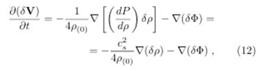
where cs represents the EoS parameter 

As from CMB blackbody spectrum

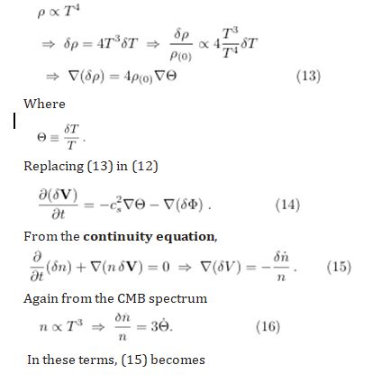
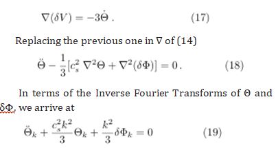
In relativistic analysis we must consider the action of gravitational redshift on the law of temperature evolution. Such action can be modeled according to the addition ad hoc, in (19), of some term such that it cancels when added to it.

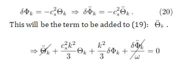
Thus, the term δΦ/ω corresponds to a variation in temperature due to the gravitational redshift suffered by the CMB 

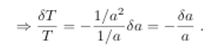
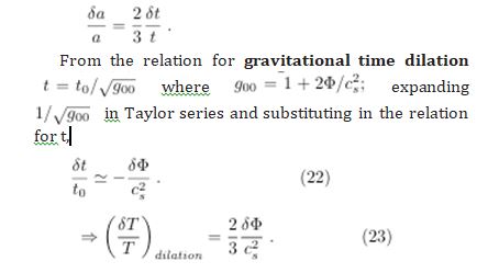
A Dilatation (Gravitational) of Time

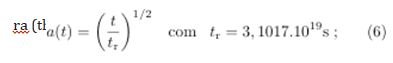
Consider, in the matter era, a(t) ∝ t2/3 and T ∝ 1/a.

On the other hand,

Interms of (21) and (23), we can estimate a total temperature deviation: the SWE

This last result corresponds to the well-known SWE: CMB photons being redshifted (losing energy) as if they were climbing some potential barrier.

If there are scalar fluctuations in the metric, what is the effect of these fluctuations on the CMB spectrum?

Let the metric FLRW spatially “flat” (κ = 0) and scalarly perturbed 

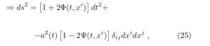
where “Φ” represents the gravitational potential at the Newtonian limit and “Ψ” a change in the metric due to the curvature of space, it comes to

The relation that describes the temporal evolution of the Boltzmann distribution function on the “mass shell” f(t, xj, Pj) is called the Boltzmann Equation (BE)

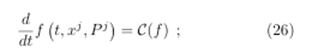
where there corresponds to C(f) some kinetic term to be adjusted according to the adopted cosmological model.

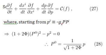
we expanded the previous relation in a power series up to the 1st order in Φ

Finally, considering only zero-order terms, by implementing this we reach the second term on the left of the approximation (27).

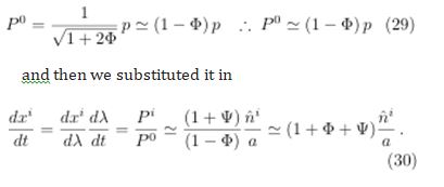
Let us now calculate the term dp/dt of (27). Starting from geodetic equation in terms of the same arbitrary affine parameter λ under the

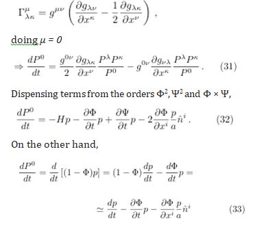
in which the relationship to dxi/dt was used. Equaling this to the derivative of (29) and taking the result in (27) considering f independent of xi (isotropy),

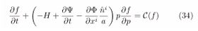
In this configuration

• H corresponds to the loss of energy due to the expansion of the Universe (zero-order term);
• +∂Ψ/∂t corresponds, in terms of the metric de- scribed in form (25), to the ”deviation” in energy due to the temporal variation of the perturbative term Ψ;
• -(∂Φ/∂xi)(nˆi/a), finally, corresponds to the spatial variation of gravity due to variations in matter density: photons ”lose” energy ”climbing potential (gravitational)” barriers”; and ”gain” energy by ”falling” into potential wells.

The Disturbance In T

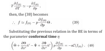
For a relativistic gas of bosons (photons are bosons) in thermodynamic equilibrium, the distribution function f(0) takes the form

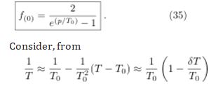
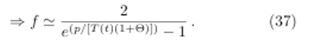
by construction, the temperature fluctuation function

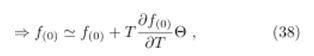
Thus, in terms of Θ, the function f(0) can be described in approximate form

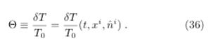
As it is known that δT/T0 ? 10−5, the previous ratio, expanded in a series of powers around T0, can be described by

where f(0) is the Bose-Einstein distribution function (35). Taking into account, also, that in zero order,

Decoupling Matter-Radiation: C(F(0) ) = 0: Immediately after the recombination phase, the uncoupled photons of matter start to propagate with an average free path of the order of + ∞, i.e., without interacting with anything else. In terms of the perturbed BE, this condition corresponds to fixing C(f(0) ) = 0.

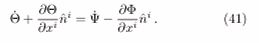
In these terms, the linearly perturbed BE (40) implies

Adopting this convention, the inverse Fourier transform (see appendix A) of the previous one is

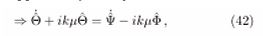
where  was defined as the cosine of the angle between the wave vector k and the direction of propagation of the photon n2.

Properly rearranged the Boltzmann equation can be described in the form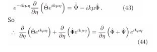 

- SWE & ISW

Integrating the previous relation into the period from recombination (ηr ) to the present tense (η0 )

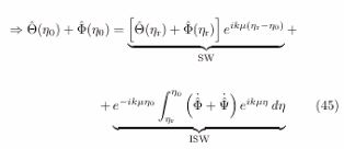
The exponential factor in the previous [equation] represents the phase shift in the photon wavefronts; this shift should be disregarded in the present approach.

The equation above represents anisotropies in the CMB temperature spectrum observed today in terms of the anisotropies at the time of recombination.

In very dense regions and under the Newtonian gauge , justifying the observed temperature fluctuation being (δT/T0) > 0. This corresponds to the pho- ton being redshifted (losing energy:“cooling”) as if it were climbing some potential barrier.

Note that, disregarding the term ISW, the expected result is recovered in the 1st order of Φ:

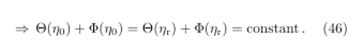
This effect corresponds to the SACHS-WOLFE EFFECT (SWE) in its simplified form.

In these exact same terms it can be seen, from the previous relationship, that the temporal variation of Φ in the period that goes from tr to t0 also modifies the temperature spectrum of the CMB. This type of anisotropy corresponding to the spectrum of the CMB is called INTEGRATED SACHS-WOLFE EFFECT (ISW).

Starting from the Euler equation describing a gravitationally disturbed fluid of photons, we arrive, having established the blackbody conditions on the photons, whereby they undergo redshift due to the Φ perturbation during the LSS. The time dilation resulting from this same disturbance increases the temperature over time (blueshift). The resulting effect of the composition of these two processes (redshift in LSS plus time dilation) on the temperature spectrum of the CMB points to the photons cooling over time: the SWE.

1. Einstein A. Die Feldgleichungen der Gravitation. Sitzungsber. Preuss. Akad. Wiss. Berlin (Math Phys). 1915: 844-847.
2. Friedmann A. Über die Krümmung des Raumes. Zeitschrift fu¨r Physik. 1922; 10: 377-386.
3. Lemaˆ?tre G. Un Univers homogène de masse constante et de rayon croissant rendant compte de la vitesse radiale des nébuleuses extra- galactiques. Annales de la Soci´et´e Scientifique de Brux- ells. 1927; A47: 49-56.
4. Robertson HP. Kinematics and World-Structure. Astrophysical J. 1935; 82: 284-301.
5. Walker AG. On Milne’s Theory of World-Structure. Proceedings of theLondon Mathematical Society, Series. 1937; 42: 90-127.
6. Sachs RK, Wolfe AM. Perturbations of a Cosmological Model and Angular Variations of the Microwave Background. APJ. 1967; 147: 73.
7. Trevisani Sergio. General Relativity, Thermodynamic Equilibrium,and Physical Cosmology.
8. Trevisani SRG, Lima JAS. Gravitational matter creation, multi-fluid cosmology and kinetic theory. The European Physical J C. 2023.
9. Trevisani Sergio. Gravitational Matter Creation in the Accelerated Expanding Universe.
10. Lima JAS, Trevisani SRG, Santos RC. Cosmic “adiabatic” photon creation: Temperature law and blackbody spectrum. Physics LettersB. 2021; 820: 136575.
11. Landau LD, Lifshitz EM. Fluid Mechanics, Second Edition: Volume 6 (Course of Theoretical Physics). Butterworth-Heinemann. 1987.
12. Bernstein J. An Introduction to Cosmology. Prentice Hall. 1998.
13. Dodelson S. Modern Cosmology. Academic Press, San Diego. 2003.
14. Multamaki T, Elgaroy Ø. Astron. Astrophys. 2004; 423: 811.
15. Shirley Ho, Christopher Hirata, Nikhil Padmanabhan, Uros Seljak, Neta Bahcall. Correlation of CMB with large-scale structure. I. Integrated Sachs-Wolfe tomography and cosmological implications. Phys Rev D. 2008; 78: 043519.
16. Kofman LA, Starobinsky AA. SvA. 1985; 11: 95.
17. So?tan AM. ISW in ΛCDM or something else?. Monthly Notices of the Royal Astronomical Society. 2019; 488: 2732-2742.
18. Benjamin R. Granett, Mark C. Neyrinck, István Szapudi. An Imprint of Superstructures on the Microwave Background due to the Integrated Sachs-Wolfe Effect. Ap J. 2008; 683: L99.
19. Carlos Hernández-Monteagudo, Robert E. Smith. On the signature of z ∼ 0.6 superclusters and voids in the Integrated Sachs–Wolfe effect Free. Monthly Notices of the Royal Astronomical Society. 2013; 435: 1094-1107.
20. Rafael C. Nunes, Supriya Pan. Cosmological consequences of an adiabatic matter creation process. MNRAS. 2016; 459: 673-682.
21. Tomas Kasemets, Jan Heisig. CMB-slow. Talk at Tuesday’s “WerkstattSeminar”. 2010.
22. Hwang J, Padmanabhan T, Lahav O, Noh H. 1/3 factor in the CMB Sachs-Wolfe effect. Physical Review D. 2002; 65: 043005.
23. Martin White, Wayne Hu. The Sachs-Wolfe Effect. 1996.
24. Scott Dodelson. Modern Cosmology. Academic Press, Elsevier Science. 2003.