Data

Bangladesh household income and expenditure survey, 2016 17 (HIES 2016-17), the latest nationwide survey by Bangladesh Bureau of Statistics (BBS) using a stratified two-stage sample design and capturing data on household poverty, standard of living, health and education status, and so on from 46,080 households, is used in this study. Among 44,378 people who have reported to be working 7,602 reported that they were ill within last 30 days.

Econometric model

A multinomial logistic regression model is deployed to examine the factors responsible for self-determining delay in treatment seeking behaviour by working class comparing four distinct groups: immediate care seekers (who make visits loosing no time), seekers of treatment soon (within two days of symptom), late (within three to four days) and very late (more than four days). Empirical studies select the scale purposively in accordance to the research environment. Chen, Rizzo and Rodriguez [2] used delaying or forgoing needed treatment within a year as a dichotomous variable as they were examining its health effects among US civilian non-institutionalized population. Abuduxike et al. [1] used the same definition for a 5-year span for people of Northern Cyprus. In contrary, Romay-Barja et al. [23] defined delay whenever treatment was sought beyond 24 hours of symptoms as they were judging the case of Malaria in Equatorial Guinea. For urinary incontinence among Chinese women a longer delay was defined by Wu et al. [24] if there was no treatment seeking within 3 years. Rucker, Brennan and Burstin [12] used number of days symptoms were persisting to define four groups: 0 days, 1-2 days, 3-6 days, and ≥ 7 days as they were examining delay in seeking emergency care in five international hospitals.

The socio-demographic approach to healthcare utilization behavior, as addressed by Anderson [25], highlights its determinants as age, sex, education, occupation, ethnicity, socioeconomic status, and income [26, 27]. However, Bice, Eichhorn, and Fox [28] found income as a determining factor only among children and adults. Andersen and Benham [29] and Richardson [30] showed how financing method influence the lower-class healthcare. Particularly Andersen and Benham [29] shows positive impact of insurance coverage on healthcare demand by low-income groups. Working with the social psychological approach Stoeckle, Zola and Davidson [31] showed how patient’s knowledge and beliefs about his/her symptoms, expectations regarding health services and understanding about need for professional care influence his/her treatment seeking. Bloom and Wilson [32] also focused patient-practitioner relationships in explaining demand for healthcare. We define our objective function incorporating our theoretical understanding and empirical deduction as:

the difference between return from investment in treatment and their loss of earnings in that period. If we assume that health investments completely revive worker illness or injury, then the treatment cost for a specific illness or injury, hi , is required to regain worker i’s daily earnings, yi . The term, (y i – h i ), therefore, indicates the benefit from treatment. Age, level of education, gender and need for regular medication are the health indicators (Xi ) included. Health, precisely health deficits, has close relationship to age [33] while education and income have significant influence on healthcare seeking [34]. Women and children are often having significant higher delay. Pre-existing health issues make people more concerned about their condition [2]. A set of person specific control variables like marital status, injury as a serious type of illness, respiratory disease as a long term illness and whether he/she received treatment from a formal healthcare provider is considered in X. Chen, Rizzo, and Rodriguez [2] considered marital status of the patient as a control variable when they were examining influence of cost issues on treatment delays. Researches on cancer, urinary diseases and as such found more patients reporting in delayed manner due to different socioeconomic factors [35,24]. Rucker, Brennan, and Burstin [12] showed that treatment delay decreases significantly depending on patient’s perception about seriousness. We have included whether a person is suffering any respiratory disease as this often requires a long-term treatment contrary to injuries that may force rushed visits to healthcare centers. Rucker, Brennan, and Burstin [12] also showed that patients make delay if they do not have a regular physician. A community variable qij identifies whether the worker i is working in a rural location (j = 1 if works in a rural area, 0 otherwise). People show differentiated behaviors towards healthcare seeking based on rural-urban differences. First, healthcare facilities are mainly urban centered. Second, physician absenteeism, faulty facilities and deficiency of treatment tools and medicine are common in rural care centers.

Endogeneity issues

The supply side of health care service suffers a great degree of asymmetric information as physicians solely determine the amount of care needed. However, this could be a possible source of biasness in any attempts of examining health care demand in Bangladesh. First, doctors’ decisions about medical care are often influenced by the socioeconomic status of their patients. Second, there can be a general mistrust about the efficiency of doctor’s opinion (both cost and outcome) among patients. Bangladesh records high and fast accelerating health tourisms. Also, wealthy people rarely trust the public health care service. Thus, the interaction between health seeking behaviour and benefit from treatment is likely to be influenced by patient’s perception about healthcare service, workplace dynamics and community attitude towards health. Because we have included only the working people the health behavior of co-workers should be the strongest [36]. According to Rucker, Brennan, and Burstin [12] personal belief about seriousness of a disease, perception about need for treatment and confidence on healthcare service are key factors for treatment delay. Not only that peer effects contribute majorly in constructing individual perception but also influence different workplace constraints that may defer treatment. The problem is that in one hand the ability to perceive and the earning capability are closely related and in the other information from the peers about healthcare providers’ quality, care process, drug, and as such have impact on treatment cost. In order to address this likely endogeneity in our model where the dependent variable is categorical, we designed a two-stage residual inclusion (2SRI) regression method following Terza, Basu, and Rathouz [37]. IV Probit and Bivariate Probit are two popular methods for correcting endogeneity in probabilistic models, the first one works better when endogenous variable is continuous and the second one is applied to models without proper instrument. However, none of these methods are applicable to models with categorical dependent variable. 2SRI and Bivariate Probit were compared in Galárraga et al. [3], finding satisfactory results from both. We define the auxiliary function as:

Galárraga et al. [3] used an asset index as a proxy for household wealth and an area specific deprivation index to control well-being at the local level when they were examining appropriateness of health insurance among Mexican poor. We have used two variables: a dummy ‘test’ that takes the value 1 if the worker had to go through any pathological laboratory test during treatment and 0 otherwise; and a continuous variable ‘travel time’ that measures the travel time to the healthcare provider. Medical check-up expresses the severity of the problem along with worker’s awareness. However, tests are done after first visit to physician or healthcare provider. Travel time expresses the transportation constraint and thereby shows worker’s unwillingness to visit healthcare provider. Unfortunately, the auxiliary function can be a secondary source of endogeneity due to its resemblance to wage function. It has a Mincer [38] type wage – human capital gradient that suffers unknown ability, household optimization and measurement impacts [39]. Including proxy measures through education of parents or spouses, physical health status, nutrition, and so on [40,41] can be one remedy of this problem. Parental education, occupation, family size, distance to school, ownership of assets and as such are used as instruments by several researchers to address endogeneity problem through instrumental regression technique [42]. We have used current market value of residence as a proxy variable for level of education based on both informal method of R-squared criteria and a penalized likelihood test [43 48]. However, because of limited options we only had to compare the selected proxy against parental education.

Variable description

More than 72% of Bangladeshi ill workers take the risk of not rushing to healthcare centers. Almost 30% of them were found making delays beyond 3 days and around 21% wait more than 5 days. Among 7602 workers who have received treatment due to illness or injury the average daily income was about BDT 319 and cost of treatment was about BDT 825. Their average age was more than 29 years, more than 52% of them were male, more than 60% were married and more than 42% required any medicine regularly. 457 of these workers were suffering from any respiratory diseases while 212 were injured. More than 36% workers received treatment from formal healthcare center, more than 43% had pathological laboratory tests and more than 64% were working in rural areas. More than 11% could not reach any healthcare within 1 hour. Around 43% workers were illiterate, 16% had received primary education and 30% had completed secondary school. Most of the workers live in cheap houses. About 2177 lived in houses worth less than BDT 100000. 

Current statistical procedures implemented in statistical software packages for the aggregation of diagnostic test accuracy data include hierarchical regression and the bivariate random-effects meta-analysis model. However, these models do not report the overall mean, but rather the mean of a central study and have differences in estimating the correlation between sensitivity and specificity when the number of studies in the meta-analysis is small and/or when the variance between studies is relatively large.

Generally, to capture the possible dependence between diagnostic test results, a binary covariance structure is assumed, but in this article, we consider the use of structures that can be modeled using copula functions as an alternative to dependence modeling with software that is readily available. A posteriori statistics of interest are obtained using Markov Chain Monte Carlo. The results obtained using our approach are compared with those obtained using models that assume bivariate structure and with those obtained using models under the assumption of independence between test results for clinical diagnosis. To illustrate the application of the method and to make comparisons, data from a study published in the literature were used.

Copula function, Binary covariance, Bayesian hierarchical model, Markov chain monte carlo, Meta-analysis, Diagnostic test.

Pambabay Calero JJ, Bauz Olvera SA, Sánchez García AB, Nieto-Libreros AB, Galindo VP (2020) Modeling for Meta-Analysis of Diagnostic Tests of Binary Responses: An Approach from Copulas and Hierarchical Models. Ann Biom Biostat 5(2): 1036.

MCMC: Markov Chain Monte Carlo; AUC: Area Under the Curve; HSROC: Hierarchical Summary Receiver Operating Characteristic; BRMA: Bivariate Random-effects Meta-analysis; Se: Sensitivity; Sp: Specificity; TP: True Positives; FP: False Positives; FN: False Negatives; TN: True Negatives; AUDIT-C: Alcohol Use Disorder Identification Test - Consumption

The exponential growth of medical literature and the increasingly widespread use of information and communication technologies, together with the dispersion of scientific literature, make it difficult for researchers, and above all health professionals, to access relevant information. Meta-analysis is a systematic review that incorporates a statistical strategy to integrate the results of several studies into a single estimate.

The correct diagnosis of an alteration is of eminent and principal interest in psychology and medicine. Diagnostic tests are common tools to discern the presence or absence of a condition or to examine patients who are at risk of developing a disease. Many diagnostic tests are based on scores obtained from brief questionnaires or are based on a single biomarker. Therefore, they will not always give a correct diagnosis. When primary studies are available that evaluate the quality of a diagnostic test, performing a diagnostic meta-analysis has become a key tool for investigating available information about a diagnostic test [1,2]. In a primary diagnostic study, the quality of a diagnostic test is often measured in terms of the sensitivity (true positive rate) and specificity (true-negative rates = 1 - false-positive rate) of the test. In order to be able to operate with likelihood ratios in the calculation of probabilities, these must be transformed into advantages (odds), these calculations are simplified by using nomograms [3]. Sensitivity and specificity vary depending on the cut-off point used to separate the presence or absence of the condition of interest. In these cases, the results can be represented graphically as a ROC curve, which allows the characteristics of the test to be known according to different cutting points and which can be used to choose the most appropriate one. An estimator of the overall relevance of a test can be the Area under the Curve (AUC). It must be borne in mind that the information available on the validity of diagnostic tests comes from different populations.

Therefore, the estimates obtained in these studies are subject to random variability and if the studies have been designed incorrectly, to biases. The variability of the measurements will be influenced by multiple factors that are of interest to know and control. Among them, it is especially important to distinguish the intra and inter-study variations.

Due to this particularity, the bivariate nature of the data must be preserved, modeling sensitivity and specificity together. Two models have been established in recent years: a hierarchical model [4], a bivariate model [5]. These models, when focusing on estimating meta-analytic sensitivities and specificities, has the advantages of accessing the individual data and of allowing unexplained heterogeneity as well as correlation between sensitivity and specificity. Moreover, it can be generalized to model covariates and can cope with extreme values of 100% for sensitivity and specificity without applying artificial continuity corrections, and standard software (e.g., R) can be used for analysis. However, there are also some disadvantages of these models. It does not operate on the original scale of sensitivity and specificity, but on the corresponding logit scale and by generally relying on the bivariate normal distribution for the random effects, it only allows one single correlation structure. Recently, a mixed copula model has been proposed as an extension of the generalized linear mixed model-GLMM [6], using a copula representation of the distribution of random effects with normal marginal and beta, respectively.

We propose here a copulas approach for the meta-analysis for diagnostic accuracy studies, which avoids the previously mentioned problems, while keeping all advantages of the Hierarchical Summary Receiver Operating Characteristic (HSROC) and Bivariate Random-Effects Meta-Analysis (BRMA) models. It uses the idea of having marginal beta distributions for sensitivity and specificity, resulting in corresponding marginal beta-binomial distributions for true positives and true negatives, and linking the marginal by copula distributions. Copulas are a useful way to model multivariate data as they explain the dependence structure between sensitivity and specificity by providing a flexible representation of a multivariate distribution. The theory and application of copulas have become important in finance, insurance, and other areas. In this article, with the help of the statistical software R [7] (R Development Core Team 2013), we compare the performance measures of the Bayesian approach against the classic bivariante model [5] using the copulation functions.

In general, meta-analysis is a two-stage process. In a first step, the results of each study are estimated, although, in the case of the evaluation of diagnostic tests, each study is summarized by a pair of indices that describe the validity of the test.

Typically, these two indices are either sensitivity and specificity, or the positive and negative likelihood ratios. In a second step, global validity indices must be calculated for which various methods have been proposed, which will be explained later. In diagnostic tests, the assumption of methodological homogeneity in the studies are not met and it is therefore important to evaluate heterogeneity.

Evaluation of heterogeneity

Assessing the possible presence of statistical heterogeneity in the results can be done (in a classical way) by presenting the sensitivity and specificity of each study in a forest plot. In these graphs, the estimators of the indices are represented together with their confidence intervals, and they are usually presented paired and ordered according to one of the indices. A characteristic source of heterogeneity is that which arises because the included studies may have used different thresholds to dene what a positive result is. This effect is known as the threshold effect.

Threshold effect

To explore this source of variation it is useful to represent in a graph the pairs of sensitivity and specificity of each study in a ROC plane. In this plane, the zone closest to the upper left corner assumes good diagnostic performance while the central zone, the diagonal in which sensitivity and specificity are equal, represents a null diagnostic capability. If there were a threshold effect, the points in the ROC space would reflect a curvilinear curve. Changing the positivity threshold of a test would result in a higher (or lower) sensitivity with the consequent opposite effect on specificity.

The most robust statistical methods proposed for meta analysis take into account this correlation between sensitivity and do so by estimating a summary ROC curve (SROC) of the included studies. However, on limited occasions the results of the primary studies are homogeneous and the presence of both threshold effect and other sources of heterogeneity can be ruled out. In this situation, the overall result of the review could be obtained from the weighted combination of the indices of the individual studies. As always, this combination can be done using either a fixed-effect model or a random-effects model, depending on the magnitude of heterogeneity. Several statistical methods for estimating the SROC curve have been proposed. The first, proposed by [8] (Moses, Shapiro & Littenberg 1993), is based on estimating a linear regression between two variables created from the validity indices of each study.

Bivariate and hierarchical approach

The Moses model has some limitations. On the one hand, it does not take into account the different precision with which sensitivity and specificity were estimated in each study, nor does it incorporate heterogeneity between studies. To overcome these limitations, more complex regression models have been proposed. The first is a bivariate random-effects model [5] (BRMA), which assumes that the logit of sensitivity and specificity follow a bivariate normal distribution.

The model contemplates the possible correlation between both indices, models the different precision with which sensitivity and specificity have been estimated, and incorporates a source of additional heterogeneity due to variance between studies. At the study level, this model assumed that the true positives and false positives within study  follow binomial distributions. At the between-studies level, a bivariate random effects model is assumed for  and  where normal priors are assumed for the study-specific parameters:

The second model refers to the Hierarchical Summary Receiver Operating Characteristic (HSROC) or hierarchical model [4]. It is similar to the previous model, except that it makes explicit the relationship between sensitivity and specificity across the threshold. The model included random effects for the cut-off and the test accuracy and focused on estimating the SROC curve. At the study level, it is assumed that within study  the True Positives (TP) and the False Positives (FP) follow binomial distributions:

where index 1 denotes diseased individuals and index 2 denotes non-diseased. The authors parameterized the sensitivities and specificities as follows:

where   is the random threshold in study i, αi is the random accuracy in study i, and is a shape (asymmetry) parameter. Normal distributions are used to model variation in the study specific parameters across studies: 

The BRMA and HSROC are adjusted using the likelihood method, assuming that the transformed data are approximately normal with constant variance; however, for sensitivity and specificity and proportions in general, the values of mean and variance depend on the underlying probability.

Both hierarchical models involve statistical distributions at two levels. At the lower level, the count of the values taken from the tetrachoric tables extracted from each study is modeled using the binomial distributions and the log-odds of the proportions. At the upper level, it is assumed that the random effects of the study explain the heterogeneity in the accuracy of the diagnostic test among studies beyond what is explained by the variability of sampling at the lower level.

The Bivariate model and the HSROC model are mathematically equivalent when covariates are not available [9,10] but differ in their parameterizations. Bivariate parameterization models sensitivity, specificity, and the correlation between them directly, while HSROC model parameterization models positivity, precision, and curve shape threshold functions to define an SROC curve. Therefore, any factor affecting the probability will change the mean and variance. This implies that models in which predictors affect the mean but assume a constant variance will not be adequate.

A third model is a mixed copula model that is an extension of the general linear mixed model of [6], using rather a copula representation of the distribution of random effects with normal and beta marginal distributions [11]. (Nikoloulopoulos 2015) demonstrates that the meta-analysis of precision studies of the diagnostic test is a primary field of application for copula models since the traditional assumption of multivariate normality is invalid in this context. Joint modelling of study-specific sensitivity and specificity using existing bivariate or copula-based beta distributions overcome the difficulties mentioned above. Since both sensitivity and specificity take values in the interval space (0,1), it is a more natural option to use a beta distribution to describe their distribution across studies, without the need for any transformation. The beta distribution is conjugated with the binomial distribution and therefore it is easy to analytically integrate the random effects giving rise to the marginal beta binomial distributions.

There are a variety of statistical packages that can be used to perform the analyses described, such as SAS and Stata, which through a series of user-programmed macros make it easier to obtain the models described. The macros of Stata are called Midas, and the macro developed for SAS is called MetaDas [12]. Other specific programs for meta-analysis of diagnostic test studies are the mada, CopulaREMADA [11] (Nikoloulopoulos 2015) and HSROC libraries of the R statistical package.

The methods below are demonstrated using a data set previously published by [13], which analyzed alcohol problems in certain individuals, considering both the 10-item AUDIT and its 3-item abbreviated version (Alcohol Use Disorder Identification Test - Consumption [AUDIT-C]) accurately detect unhealthy drinking, to examine whether the AUDIT-C is as accurate as the full AUDIT in detecting unhealthy alcohol use in adults. The study estimated sensitivity and specificity values around 0.86 and 0.78 respectively.

Fourteen studies evaluating individuals with 18 332, of whom 2 071 had alcohol problems, were included in the review. The prevalence of studies ranged from 5% to 37%, with a median of 11%, (Table 1).

A statistical method for meta-analysis of diagnostic tests from a copula approach

Copula is a well-known statistical concept for modeling dependence on random variables. A copula is a joint distribution function whose marginal are all uniformly distributed and can be used to model the dependence separately from the marginal distributions, i.e., it is a function that approximates the set behavior of random variables from their individual behaviors [14]. Two random variables  and  with distribution function  and , (Sklar 1959) demonstrated that there is a C function can be written as:

where  is itself a distribution function for a bivariate pair of uniform random variables and  ) 1 2 , function for the original variables   and  Therefore, a bivariate copula is a function that fulfills the following properties [15] (Nelsen 2007): 

The concept of copula allows modeling the dependence between marginal distributions through the copula parameters. That is to say, in the present paper we will use only a parametric model, despite the fact that there are non-parametric copulas that can be used in order to model the dependence between random variables.

These association parameters can be transformed in correlation measurements, such as the Spearman or Kendall correlation coefficients. [16] (Schweizer, Wol et al. 1981), showed that both measurements can be used for the description of dependence.

where 12 c denotes the density of a bivariate copula. Density is treated as a plausibility function. Note that in the case of copula, the likelihood is determined analytically and has a closed form. Therefore, the standard methods of maximum likelihood are used for parameter estimation. An advantage of the copula model is that, in principle, there are a large number of copula that allow for different association structures. This is in contrast to the standard model where a bivariate normal distribution is used as a single correlation structure. There are a rich number of copula that can be used, each resulting in a new model for the meta-analysis of precision diagnostic studies. To be specific, we use the following copulas, the bivariate copula Gaussian, Clayton and Frank, these are copulas that can be adjusted to Equation 11 [11] (Nikoloulopoulos 2015).

Selection of a Model Copula

The aim is to identify among the copula families set out in previous section, which family or families best fit the joint distribution of i Se and i Sp. This is done using the Cramér-von Mises goodness-of-fit test [18] (for details of this test.

Simulation Study

A simulation study was carried out to compare the adjustment of the different copulas. The scenario specifications were designed to reproduce realistic situations found in the meta-analysis of diagnostic accuracy studies.

Generation of simulated data and goodness-of-fit of copulas models

Meta-analyses were investigated with different numbers of studies at random (k = 5; 10; 20; 35). The size of a study in each meta-analysis, nj , were randomly sampled from a uniform distribution, U(30; 1 255); given an underlying prevalence, p, individuals within each study were randomly classified as sick or undiagnosed, and a continuous test result value, x, was assigned and randomly sampled [19]. To determine the corresponding tetrachoric tables, the package Copula Remada of the statistical program R was used, using the function rCopula REMADA. beta.

To create the 2x2 table for each study, individuals were classified as a true positive, false negative, false positive, or true negative based on the test result and disease status. The sensitivity and specificity of the studies was adjusted by a uniform distribution with parameters 0:8 and 1. We generated 21 011 studies in 10 58 independent meta-analysis datasets to allow a reliable analysis of the goodness of fit of previously analyzed models. The goodness-of-fit of copulas models was assessed by examining the test statistician’s estimates and the p-value of the statistical test proposed by [18].

Adjusting The Hierarchical HSROC and Copula Model

We will use the CopulaDta package [20] (Nyaga, Arbyn & Aerts 2016) to adjust the copulas analyzed in Section 2.5. The package facilitates the application of complex models and their visualization within the Bayesian framework with short execution times and provides functions of binomial beta bivariate distributions built as a product of two beta marginal distributions and copula densities discussed in the previous Section.

The HSROC package is used to estimate the parameters of a hierarchical summary receiver operating characteristic (HSROC) model allowing for the reference standard to be possibly imperfect, and assuming it is conditionally independent from the test under evaluation. The estimation is carried out using a Gibbs sampler. The package consists of 4 functions. The two main functions are HSROC and HSROCSummary. HSROC, which must be run first, is used to implement a Gibbs sampler while HSROC Summary produces summaries for the HSROC model parameters. The remaining 2 functions are secondary functions: sim data simulates a dataset based on the HSROC diagnostic meta-analysis model, while beta. parameter returns the shape parameters of the  probability corresponding to a given range.

Results of the adjustment to AuditC data and simulated data

It is important to analyze the behavior and distribution of the data, before fitting any model, for our analysis, we will use statistical tests based on measures such as: chi-square, Cook distance and Mahalanobis, [21,22] Comrey 1985, Cook 1977, Rasmussen 1988). In that sense, Figure 1, shows that, there are influential studies in the BRMA modeling and that the goodness of the adjustment and bivariate normality is not adequate, particularly due to studies 3 and 8 from Table 1 (Figure 1).

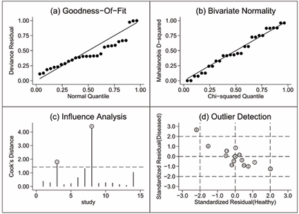
Figure 1: Goodness-of-t, bivariate normality, influential and atypical data.

On the other hand, Figure 2 shows how the different values of sensitivity and specificity are located below or above the dotted line (average), indicating a strong presence of heterogeneity in both measures.

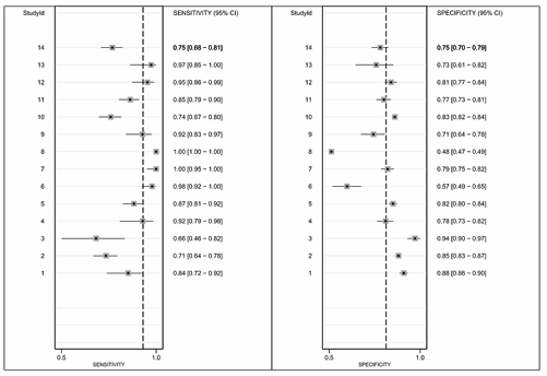
Figure 2: Foresplot.

That is, the graph demonstrates an asymmetry of the test performance means towards higher sensitivity with lower specificity, providing indirect evidence of certain heterogeneity threshold variability (Figure 2).

As mentioned above, the HSROC and BRMA models are equivalent when there is no inclusion of covariates, so we will analyze the outputs produced by the HSROC package of R. The HSROC Summary function creates plots to help evaluate whether the Gibbs sampler has converged. Each trace plot is a scatter plot of the posterior sample of a single parameter vs the iteration number of the Gibbs sampler. The trace plots for the sensitivity and specificity are shown in Appendix 1. For our example, we can see that convergence seems to be achieved fairly quickly. Another graphical summary produced by the HSROC Summary function is the density plot.

It plots a smoothed posterior kernel density function for each parameter. Appendix 2 shows density plots for some of the between-study parameters. The function also produces a summary receiver operating characteristic (SROC) curve.

The SROC curve summarizes the relationship between sensitivity and (1 - specificity) across studies, taking into account the between-study heterogeneity. The SROC curve for the Audit C data is shown in Figure 3, where, it can be noted that the values for sensitivity and specificity are: 0.430 CI95% (0-0.913) and 0.982 CI95% (0.734-1) respectively (Figure 3).

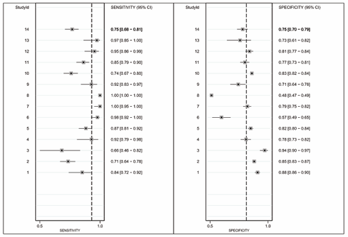
Figure 3: Foresplot.

Individual studies are depicted by a clear circle. The radius of the circle is proportional to the sample size of the study. The black circle marks the pooled sensitivity and specificity across the 14 studies in this meta-analysis. The 95% prediction region is defined by the black dotted-curve. The black dot-dashed-curve marks the boundary of the 95% credible region for the pooled estimates of sensitivity and specificity across the 14 studies. Finally, the correlation between sensitivity and (1-specificity) is 0.854. Table 2 shows that Frank’s copula is the most extreme, with a correlation of -0.600, although the Gauss and C90 models also have a high correlation whose values are -0.570 and -0.466 respectively.

It is important to note that the sensitivity and specificity results for the Auditc data in the copula models (sensitivity between 0.85-0.87 and specificity between 0.75 0.76) are very close to the values provided by [13]. That is, the estimates made by copulas are more reliable than the estimates made by the HSROC model (very low sensitivity 0.430 and very high specificity 0.98) (Table 2) (Figure 4).

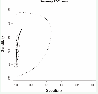
Figure 4: SROC for AuditC data.

Since the data is not distributed as a bivariate normal, and the value of the correlation between performance measures is positive, modelling of dependency through copulas should be used. In that sense, you have the results for the values of sensitivity, specificity and correlation , table 2. The algorithms used can be seen in Appendix 3.

For each copula described above, the respective goodness of-fit tests are performed. The results are shown in Table 3.

To link marginal beta distributions with a bivariate dependent distribution, the best fit is observed when working with FGM copula. This is seen in the value of the statistic and p-value which leads to the acceptance of the hypothesis of equality of empirical and parametric distributions. For FGM copulation, the value of the statistic and the p-value are 0.022 and 0.903. Note that, the p-value for FGM copula is the highest value in relation to the other copulas Table 3.

Table 4 shows the average estimates with their respective 95% confidence intervals of the statistician and the p-value of the hypothesis test for each copula model according to the number of studies simulated for each meta-analysis.

FGM copula best fits the simulated data for numbers of studies between 5 and 22, as the average value of the statistic is the lowest compared to the other copula models. Between 23 and 28 studies the best fit was achieved with Gaussian Copula and for studies between 29 and 35 the best fit was achieved with Clayton Copula (Table 4).

[In this paper, definition, implications and methodologies were presented for the development of models in the meta analysis of diagnostic tests associated with copulas, applied to a particular data set, although [23,24] pointed out that it might be difficult to estimate copulas from a data set, especially for count data. This problem may not occur under the conditions indicated in the article, because the parameter  is modeled from a continuous distribution. In general terms, copulas are functions that approximate the set behavior of random variables, based on their individual (marginal) behaviors [14].

Sensitivity and specificity measurement models that make more realistic assumptions about marginal distribution functions (e.g., those that deviate from the assumption of normality), although they may be more expensive in computational terms, are best measured by summaries of a meta-analysis of diagnostic tests. In this sense, models derived from copula offer a structure analytical flexible that is appropriate for the measurement of sensitivity and specificity.

In the meta-analysis of diagnostic tests there is great heterogeneity [25,26], due to prevalence, the number of studies, individuals analyzed, laboratory procedures, etc. For this reason, bivariate copulas can be expanded and modeled in conjunction with sensitivity and specificity using multivariate copulas.

The HSROC model does not operate on the original scale of sensitivity and specificity, but on the corresponding logit scale and by generally relying on the bivariate normal distribution for the random effects, it only allows one single correlation structure. So we propose the use of copulas for the meta-analysis for diagnostic accuracy studies, which avoids the previously mentioned problems.

The use of copulas allows the study of dependencies with structures that are not necessarily linear which is possible in diagnostic situations whose results are obtained after dichotomization. Copula models that use beta-binomial distributions to characterize the marginal of true positives and negatives are linked to bivariate or multivariate copulas, i.e., it is a bivariate logistic regression model with random effects, presenting greater flexibility to capture the functional dependence between sensitivity and specificity. In other words, hierarchical models assume a normal bivariate behavior between the logit transformations of sensitivity and specificity. When the bivariate normality assumption is not met, copula modeling is used, which uses beta-binomial distributions to characterize the marginal distributions of the true positive and negative, i.e. it presents a greater flexibility to capture the functional dependence between sensitivity and specificity.

We illustrate the procedure using a dataset published in the literature. The adjustment of the data was obtained by assuming binary associated tests and taking covariance as a parameter. It is important to note that the five copulas naturally and correctly capture the dependence structure between sensitivity and specificity (inverse relationship). The FGM copula showed a better fit compared to Gauss, C90, C270 and Frank copulas, as it obtained the highest sensitivity value. On the other hand, Frank’s copula estimated the highest correlation between sensitivity and specificity and the estimated values for the pair of summary measures (sensitivity and specificity) are very close to the values obtained by [13]. This is not the case with the HSROC method, reflecting the effect that hierarchical modeling has in capturing the relationship between sensitivity and specificity.

Likewise, from the results of the 2x2 table, it can be seen that the best modeling for the study data corresponds to the FGM copula according to the Cramér-von Mises goodness-of-fit test. In the same sense, copula modeling estimated higher sensitivity values than the HSROC model, that is, for the present context, parameter estimates by couples were better than the hierarchical model.

An attractive feature of copulas is that through beta-binomial distributions the measurements of TP and TN are modelled, which is due to the fact that the beta distribution is conjugated with the binomial distribution. An explicit advantage of the beta-binomial distribution is that study sizes are automatically accounted for and the relationship between sensitivity pair and specificity is captured naturally. These characteristics do not happen with the BRMA model, other words, modeling by copulas is a true random effects model, which means that all tests within studies have a single specific parameter (Se; Sp).

For the selection of a dependent bivariate copulation model, the use of hypothesis tests fits highlighted easy to understand. This allows analysts too quickly and identifies a copula model for the construction of a bivariate dependent distribution that fits a data set well.

We have simulated meta-analysis in several scenarios (different numbers of studies, etc) and evaluated the hierarchical model of copulations. The methodology presented allows us to identify the best fit for the copulas analyzed in this work. It suggests that for several studies between 5 and 22, the FGM copula performs the best fit.

To finally conclude, the proposed model with marginal beta-binomial distributions and bivariate copulas seems to be a promising tool for the meta-analysis of diagnostic accuracy studies. What are probably needed in the future are feasible model selection tools that help to assess fits of different models to data sets. These tools should be able to discriminate between the hierarchical models and the copula models but also between different copula models. Until then, it might be a good idea to compute the copula models along with the hierarchical models to check the robustness of the latter.

The authors declare that there is no conflict of interest regarding the publication of this paper. The first author’s research was supported by financial assistance from Escuela Superior Politécnica del Litoral, Ecuador. The second author’s research was supported by financial assistance from Escuela Superior Politécnica del Litoral, Ecuador.

1. Egger M, Smith GD, Schneider M. “Systematic Reviews of Observational Studies,” in Systematic Reviews in Health Care, London, UK: BMJ Publishing Group. 2001; 211-227.

2. Hasselblad V, Hedges LV. Meta-analysis of screening and diagnostic tests. Psychol Bull. 1995; 117: 167-178.

3. Fagan. Nomogram for Bayes’s theorem. N Engl J Med. 1975; 293: 257.

4. Rutter CM, Gatsonis CA. A hierarchical regression approach to meta analysis of diagnostic test accuracy evaluations. Stat Med. 2001; 20: 2865-2884.

5. Reitsma JB, Glas AS, Rutjes AWS, Scholten RJPM, Bossuyt PM, Zwinderman AH. Bivariate analysis of sensitivity and specificity produces informative summary measures in diagnostic reviews. J Clin Epidemiol. 2005; 58: 982-990.

6. Chu H, Nie L, Chen Y, Huang Y, Sun W. Bivariate random effects models for meta-analysis of comparative studies with binary outcomes: Methods for the absolute risk difference and relative risk. Stat Methods Med Res. 2012; 21: 621-633.

7. RDC Team. R: A language and environment for statistical computing. 2011.

8. Moses LE, Shapiro D, Littenberg B. Combining independent studies of a diagnostic test into a summary roc curve: Data-analytic approaches and some additional considerations. Stat Med. 1993; 12: 1293-1316.

9. Arends LR, Hamza TH, van Houwelingen JC, Heijenbrok-Kal MH, Hunink MGM, Stijnen T. Bivariate Random Effects Meta-Analysis of ROC Curves. Med Decis Mak. 2008; 28: 621-638.

10. Harbord RM, Deeks JJ, Egger M, Whiting P, Sterne JAC. A unification of models for meta-analysis of diagnostic accuracy studies. Biostatistics. 2007; 8: 239-251.

11. Nikoloulopoulos AK. A mixed effect model for bivariate meta-analysis of diagnostic test accuracy studies using a copula representation of the random effects distribution. Stat Med. 2015; 34: 3842-3865.

12. Takwoingi Y, Deeks J. METADAS: A SAS macro for meta-analysis of diagnostic accuracy studies User guide version 1.3. 2010; 37.

13. Kriston L. Meta-analysis: Are 3 Questions Enough to Detect Unhealthy Alcohol Use? Ann Intern Med. 2008; 149: 879-888.

14. Ghalibaf MB. Relationship between kendall’s tau correlation and mutual information. Rev Colomb Estad. 2020; 43: 3-20.

15. Nelsen R. An introduction to copulas. Springer Science & Business Media. 2007.

16. Schweizer B, Wolff EF. On Nonparametric Measures of Dependence for Random Variables. Ann Stat. 1981; 9: 879-885.

17. Kuss O, Hoyer A, Solms A. Meta-analysis for diagnostic accuracy studies: a new statistical model using beta-binomial distributions and bivariate copulas. Stat Med. 2014; 33: 17-30.

18. Haigh J, Conover WJ. Practical Nonparametric Statistics. J R Stat Soc Ser. 1981; 144: 370.

19. Bachmann LM, Puhan MA, Ter Riet G, Bossuyt PM. Sample sizes of studies on diagnostic accuracy: Literature survey. Br Med J. 2006; 332: 1127-1129.

20. Nyaga VN, Arbyn M, Aerts M. CopulaDTA: An R Package for Copula Based Bivariate Beta-Binomial Models for Diagnostic Test Accuracy Studies in a Bayesian Framework. 2016.

21. Cook RD. Detection of Influential Observation in Linear Regression. Technometrics. 1977; 19: 15-18.

22. Rasmussen JL. Evaluating Outlier Identification Tests: Mahalanobis D Squared and Comrey Dk. Multivariate Behav Res. 1988; 23: 189-202.

23. Genest C, Nešlehová J. A Primer on Copulas for Count Data. ASTIN Bull. 2007; 37: 475-515.

24. Mikosch T. Tales and facts-rejoinder. Extremes. 2006; 9: 55-62.

25. Chu H, Nie L, Cole SR, Poole C. Meta-analysis of diagnostic accuracy studies accounting for disease prevalence: Alternative parameterizations and model selection. Stat Med. 2009; 28: 2384 2399.

26. Calero JJP, Bauz-Olvera SA, Nieto-Librero AB, Villardón MPG, Hernández-González S. An Alternative to The Cochran-(Q) Statistic For Analysis Of Heterogeneity In Meta-Analysis Of Diagnostic Tests Based On Hj Biplot. Investig Operacional. 2018; 39: 536-545.