Nonparametric Dynamic Bayesian Networks Approximate Protein Interaction Networks in a Simulation Study

Yessica Y Fermín R; Katja Ickstadt

doi:10.47739/1031

Nonparametric Dynamic Bayesian Networks Approximate Protein Interaction Networks in a Simulation Study

Research Article | Open Access | Volume 5 | Issue 1

Article DOI : https://doi.org/10.47739/2374-0116/1031

Yessica Y Fermín R¹ Katja Ickstadt^2*

^1. Independent Scientist, Colombia
^2. Department of Statistics, TU Dortmund University, Germany

+ Show More - Show Less

Corresponding Authors

Katja Ickstadt, Department of Statistics, TU Dortmund University, 44227 Dortmund, North Rhine-Westphalia, Germany, Tel: +492317553120; Fax: +49-231-755-5303;

Abstract

A cellular function emerges from a collective action of a large number of proteins interacting and affecting each other. A major challenge in the recognition of protein interaction networks is the cell-to-cell heterogeneity within a sample. This heterogeneity hampers the usage of single parametric models that cannot handle population mixtures, such as Bayesian networks, artificial neural networks, and differential equations. A nonparametric alternative is proposed by [1] in 2011, the nonparametric Bayesian network method. An extension of the nonparametric Bayesian network method is here presented by using Gaussian dynamic Bayesian networks. This allows the possibility of an analysis considering both cell-to-cell variability and temporal correlations between interacting proteins. In our results, we show that our new method called nonparametric dynamic Bayesian network method significantly improves the nonparametric Bayesian network method for the analysis of protein time series and its results are consistent.

Keywords

Gaussian dynamic Bayesian networks; Heterogeneous cell populations; Nonparametric Bayesian mixture models; Systems biology; Temporal correlations.

CITATION

Yessica Y Fermín R, Ickstadt K (2020) Nonparametric Dynamic Bayesian Networks Approximate Protein Interaction Networks in a Simulation Study. Ann Biom Biostat 5(1): 1031.

ABBREVIATIONS

ANN: Artificial Neural Network; AUROC: Area under the ROC Curve; ASW: Average Silhouette Width; BN: Bayesian Network; GDBN: Gaussian Dynamic Bayesian Network; MCMC: Markov Chain Monte Carlo; ML: Machine Learning; NPBN: Nonparametric Bayesian Network; NPDBN: Nonparametric Dynamic Bayesian Network; NPBMM: Nonparametric Bayesian Mixture Model; PCO: The percentage of correctly allocated observations; ROC: Receiver Operating Characteristic Curve

INTRODUCTION

A cellular function emerges from a collective action of a large number of proteins interacting and affecting each other. Many of these interactions are randomly produced and, therefore, the protein interaction network is still unknown. In some works, machine learning (ML) methods [2], among others, differential equations [3,4], and Bayesian networks (BNs) [5,6] have been applied to address this issue. Among applied ML methods, artificial neural networks (ANNs) have been found to be very effective for discovering protein interactions (see, e.g., [2]). However, ANNs as well as differential equations do not allow capturing in more detail the regulatory relationships in the network, as, for example, the direction of regulation. Other disadvantages of differential equations are the well-known complexity in the computation as well as the requirement of a priori knowledge of kinetics parameters associated with the interactions between proteins. Instead, methods based on BNs, as Gaussian Bayesian networks (GBNs), employ a probabilistic mechanism for the identification of protein interactions, which requires only the quantification of protein levels in a molecular sample. Furthermore, the BN graph used to represent the relationships among variables makes it fairly understandable to the researcher.

A major challenge in the reconstruction of protein interaction networks is the cell-to-cell heterogeneity within a sample, due to, among others, genetic and epigenetic variabilities (see [7] and references therein). This heterogeneity hampers the usage of a single parametric model like those mentioned in the previous paragraph and many lead to invalid interactions due to lack of adjustment. To address this issue, some studies such as [7,8] have suggested the previous identification of cellular subpopulations using mixture models for a later estimate of the protein interaction networks. In that respect, [8] uses mixtures of ordinary differential equations, while in [7] a nonparametric Bayesian mixture of Gaussian BNs, also known, and mentioned here, as nonparametric Bayesian networks (NPBNs), was employed. Both works, [7] and [8], showed the success of using mixture models in conjunction with the recognition of protein interactions for the classification of observations in heterogeneous cell populations. A well-known drawback of these methods is that both were developed on snapshot data of a dynamic process and, respectively, fail to capture temporal information and modeling of cyclic networks. Therefore, these methods can be applied only on type of single-cell multiparametric measurements currently available, such as multicolor flow-cytometry, multiplexed mass cytometry, and toponome imaging.

Advances in the so-called “super-resolution” protein quantification methods produce information on the dynamics of proteins, which provides at the same time an opportunity for a better understanding of protein interactions. In order to include temporal dynamics of proteins, we propose an extension of NPBNs by using Gaussian dynamic Bayesian networks (GDBNs). A GDBN is a generalization of GBNs by using a directed graph to include temporal relationships among variables, and allows feedback loops, i.e., edges pointing from a variable Xj at a time point t - 1 to a variable Xi at a time point t. In studies of biochemical networks, feedback loops can be intuitively interpreted as self-regulation or self-inhibition. Thereby, GDBNs have been also employed in the reconstruction of gene regulatory networks [9,10].

However, GDBNs cannot deal with cell-to-cell variability. In cases of heterogeneity this could lead to poorly specified interaction models. In order to overcome this limitation, we propose a nonparametric alternative by using a combination of GDBNs and nonparametric Bayesian mixture models (NPBMMs). We call here this method “nonparametric dynamic Bayesian networks (NPDBNs)”. The dynamic of cellular protein interaction networks is here described as a multivariate temporal process of first-order Markovian dependence structure in which the expression levels of two involved proteins, Xi(t) and Xj(t-1), are first-order temporal correlated. We investigate the properties of NPDBNs in a thorough simulation study, and compare them to NPBNs as well as GDBNs. Our results show that the proposed NPDBN method improves significantly over the NPBN and GDBN approaches.

MATERIALS AND METHODS

Simulation Study

Synthetic time-series protein expression data have been generated from realistic protein interaction networks by using first-order multivariate vector autoregressive models (MVARs) such as [11]:

$X_{t}=WX_{t-1}+\varepsilon _{t}$

where the dynamic process $X_{(t)}=\left ( X_{1(t)},,.....,X_{n(t)} \right ){}'$ is the set of time series of n proteins for $t\in Z$ . W is an n-by-n time-invariant matrix of weights, where the weights represent the strength of interaction between all pair of proteins; and $\varepsilon _{\left ( t \right )}=\left ( \varepsilon_{1\left ( t \right )}, \varepsilon _{2\left ( t \right )},....,\varepsilon_{n\left ( t \right )} \right ){}'$ is the matrix of additive Gaussian noises to the protein expression at time t with mean vector $\mu=\left ( \mu_{1}, \mu_{2},...., \mu_{n} \right )$ and variances $\sigma ^{2}=\left ( \sigma ^{2}_{1}, \sigma ^{2}_{2},...., \sigma ^{2}_{n} \right )$ . The evaluation of our method requires an intimate control of degradation of the interaction networks, which can be reached, so far, only through the use of the MVAR models above defined.

Our simulation study includes different parameters. As a first parameter we define the number of cell-subpopulations, which means the different underlying classes that we can find in a random cell-sample. Since we work with a number of 10 nodes (proteins) or less, the possibility to identify more than two statistically different subpopulations is small, and, we here consider mixture observations of two and four separate subclasses. The second parameter is the sample proportion, which means the number of observations in each existing subclass. Variation of this parameter enables to generate realistic situations, in which the relative abundance of different cell subpopulations is unbalanced. The third parameter, the number of nodes (or number of proteins), reflects the complexity of the network. In our simulation study we generated networks up to 10 nodes, because current measurement techniques in biological systems can measure up to 10 proteins simultaneously. The fourth parameter, the network density, models the proportion of possible connections (relationships) in the network that are present (see also definition in [12]). The last parameter to consider, but not less relevant, is the intra-cell-subpopulation variability, representing the underlying variation in protein expression levels within each cell-subpopulation. The noise level and length of time series are used to define this parameter. The noise level represents the fractional deviation from the expression level average. The noise level as well as the length of the time series can affect the recognition of the temporal relations between proteins.

For the generation of realistic protein interaction networks, we set in the simulation study the number of nodes and network density based on real protein interaction networks discussed in [12]. Under this information, the function “random.graph.game” in the R package i graph can give us network structures close to these values. More details of the simulation study can be found in Table 1, where the rows contain the parameter values varied in the simulations. Each combination of parameter values per column corresponds to a different dataset.

Table 1: List of parameters involved in the simulation study and employed values. Each combination of parameter values per column corresponds to a different dataset.
	Number of Cell-subpopulations	Sample Proportion	Network Density	Number of Proteins	Noise Level and (&) Time Series Length
Number of Cell-subpopulations	2	2	2	2	2
	4
Sample Proportion	1:01	1:01	1:01	1:01	1:01
		1:03
		1:07
Network Density	0.3	0.3	0.3	0.3	0.3
			0.6
Number of Proteins	5	5	5	3	5
				5
				10
Noise Level and (&) Time Series Length	0.1&100	0.1&100	0.1&100	0.1&100	0.1&20
					0.5&20
					0.8&20
					0.1&100
					0.5&100
					0.8&100

Nonparametric Dynamic Bayesian Networks (NPDBNs)

This section contains an extension of the NPBN method [1] for protein interaction networks. Different from NPBNs, our approach employs nonparametric Bayesian mixture models in combination with GDBNs instead of GBNs. GDBNs as mixing components allow modeling temporal dependencies, which can be of interest in the resolution of protein interaction networks. A GDBN is defined by the product of Gaussian conditional distributions of the form:

$p\left ( X_{i\left ( t \right )}|Pa_{i\left ( t-1 \right )},\beta _{i},\sigma ^{2}_{i} \right )\sim N\left ( X_{i\left ( t \right )}|\sum _{Ji} \beta _{i,j}X_{j\left ( t-1 \right ),\sigma ^{2}_{i}}\right ),$

$J_{i}=\left \{ j\in \left \{ 1,....,n \right \}|X_{j\left ( t-1 \right )}\in Pa_{i\left ( t-1 \right )} \right \}$

where the sets of parents are here denoted as $Pa_{i\left ( t-1 \right )}$ , and correspond to the set of proteins $X_{j\left ( t-1 \right )} \in X_{\left ( t-1 \right )}$ that can directly regulate a target protein $X_{i\left ( t\right )} \in X_{\left ( t \right )}$ ; the set of coefficients , $\beta_{i}=\left \{ \beta _{i,j} \right \}$ , located in the expected value of that distribution represent the weights or strength of interaction between the involved proteins in the MVAR model defined above. The unconditional variances are here denoted as $\sigma _{i}^{2}$ . Assuming a heterogeneous cell-population with K cellular subpopulations, we define a mixture model of GDBNs to approximate the joint distribution of interacting proteins as follows: $p\left ( X_{\left ( t \right )}|K,\lambda ,G,B,\sigma ^{2} \right )=\sum_{h-1}^{K}\lambda _{h}p\left ( X_{\left ( t \right )}|G_{h},B_{h},,\sigma _{h}^{2} \right )$

where K and λare the mixture model parameters, here assumed as random variables. The prior distribution of K is well defined as a geometric or a Poisson distribution, while λ is assumed to follow a Dirichlet distribution. These two parameters are the key in modeling the heterogeneity.

Moreover, a different correlation structure for each mixture component is here assumed, and G denotes a set of protein interaction networks associated with each “h” component. B is a set of regression coefficients associated with the expected values of a Gaussian joint probability distribution defined by the product of conditional distributions of form shown in Equation 2, and $\sigma^{2}$ represents the respective variances. For each component h, we have a $B_{h}=\left \{ \beta _{i,h} \right \}_{i=1}^{n}$ and a $\sigma ^{2}_{h}=\left \{ \sigma ^{2} _{i,h} \right \}_{i=1}^{n}$ that define each $G_{h}$ the directed graph of a GDBN associated with component h. This graph describes the correlations of proteins. Thus, relationships between proteins are defined by directed edges pointing from one edge to another. In a graph, the direction of edges characterizes the direction of regulation between proteins. That is, a protein that connects to another is said to regulate that protein, whereas in the case of disconnection we speak of non-adjoining temporal correlations or conditional independence between proteins.

Implementation

In the NPDBN method the classification of observations in different components is achieved by using an indicator variable, known also as allocation vector. This vector allows the assignment of the observations to their respective subclasses.

For example, in a sample denoted here as $D=\left ( D_{1},........,D_{r} \right )$ with r independent observations of a temporal multivariate process $X_{t}$ , Let $C=\left ( C_{1},....,C_{r} \right )$ be an allocation vector, where $C_{s}=h$ implies that the s-th sample, $D_{s{}'}$ is coming from the h-th mixture component. In Equation 3 the independence of components implies that observations in them are also independent, that is, $C_{s},S=1,....,r$ are independent over the K components, with $p\left ( C_{s}= h \right )=\lambda _{h}$ so that $p\left ( C \right )=\prod_{h=1}^{K}\lambda _{h}^{rh}$ where ${rh}$ is the number of samples allocated by c to component h. Conditioning Equation 3 on c, it becomes:

$p\left ( D|K,c,G,B,\sigma ^{2} \right )=\prod_{s=1}^{r}p\left ( D_{s}|G_{c_{k}},B_{c_{s}},\sigma _{c_{s}}^{2} \right )=\prod_{s=1}^{r}\prod_{i=1}^{n}p\left ( D_{si}|D_{sPa_{i}},B_{i,c_{s}},\sigma _{i,c_{s}}^{2} \right )$

where $D_{s}$ is an n-by- $m_{s}$ matrix consisting of $m_{s}$ time-dependent realizations of $X_{t}$ . $D_{si}$ and $D_{sPa_{i}}$ denote the $m_{s}-1$ realizations of the target variable $X_{i\left ( t \right )}$ and of its parent set $Pa_{i\left ( t-1 \right )}$ respectively. As all the observations within the same component belong to the same cell-subpopulation, the protein interaction network and its associated parameters are also the same. Therefore, we can rewrite Equation 4 as follows:

$p\left ( D|K,c,G,B,\sigma ^{2} \right )=\prod_{h=1}^{K}p\left ( D_{h}|G_{h},B_{h},\sigma _{h}^{2} \right )=\prod_{h=1}^{K}\prod_{i=1}^{n}p\left ( D_{hi}|D_{hPa_{i}},B_{i,h},\sigma _{i,h}^{2} \right )$

where

$D_{h}=\left \{ D_{s}\in \left \{ D_{1},...,D_{r} \right \}:c_{s}=h \right \};D_{hi}=\left \{ D_{si}\in \left \{ D_{s1},...,D_{sr} \right \}:c_{s}=h \right \};$

and $D_{hPa}=\left \{ D_{sPa_{i}}\in \left \{ D_{s1},...,D_{sr} \right \}:c_{s}=h \right \};$

$\beta _{i,h}$ are the coefficients of relations between variables involved in the interaction network of component h; and $\sigma ^{2} _{i,h}$ are the unconditional variances of variable $X_{i}\left ( t \right )$ in component h. This methodology requires the estimation of the number of distinct cell-subpopulations, allocation vector and temporal protein interaction networks associated with each component. Thus, the implementation of our approach requires the analytical integration of the parameters $\beta _{i,h}$ and $\sigma ^{2} _{i,h}$ .This integration is well known in Bayesian statistics, since models such as linear regression models are obtained in the same way. Thus, following the parametrization used in [14] we obtain that:

$p\left (X_{i\left ( t \right )}=D_{hi} |Pa_{i\left ( t-1 \right ),h}=D_{hPai}\right )=\int p\left ( D_{hi}|D_{hPa_{i}},\beta _{i,h},\sigma _{i,h}^{2} \right )p\left ( \beta _{i,h} ,\sigma _{i,h}^{2}\right )d\beta _{i,c_{s}}\sigma _{i,c_{s}}^{2}=\prod _{sh}\int p\left ( D_{si}|D_{sPa_{i}},\beta _{i,c,},\sigma _{i,h}^{2} \right )p\left ( \beta _{i,c_{s}} ,\sigma _{i,c_{s}}^{2}\right )d\beta _{i,c_{s}}\sigma _{i,c_{s}}^{2}=$

$\prod _{sh}\frac{b^{a\Gamma \left ( a+\frac{\left ( m_{s}-1 \right )}{2} \right )^{*}\sqrt{\left | V^{*} \right |}}}{\left ( 2\pi \right )\frac{\left ( m_{s}-1 \right )}{2} \Gamma \left ( a \right )\sqrt{\left | V_{\beta } \right |}}$

$\left [ b+\frac{1}{2}\left ( \mu _{\beta }^{{}' } V_{\beta }^{-1}\mu _{\beta }+D_{si}^{{}'}D_{si}-\mu ^{\left ( * \right )}\right )V^{\left ( * \right )-1} \mu ^{\left ( * \right )}\right ]^{-\left ( a+\frac{m_{s}-1}{2} \right )}$

Thus, a conditional probability of the target variable $X_{i\left ( t \right )}$ on its parent set $Pa_{i\left ( t-1 \right )}$ can be defined by integration of the main parameters, which result in a product of distinct multivariate Student´s t distributions. Subindex $S_{h}=\left \{ S\in \left \{ 1,.....,r \right \}:c_{s}=h \right \};$ describes the set of employed observations. The constants a, b, vectors $\mu _{\beta }$ , $\mu ^{*}$ ,and matrices $V_{\beta },V^{*}$ are hyperparameters associated with involved probability distributions into the integral (see [7]), which can be estimated through a simulation study here modeled. The mean vector $\mu ^{*}$ and precision matrix $V ^{*}$ are given by:

$\mu ^{*}=\left ( V_{\beta }^{-1}+D_{sPa_{i}}^{{}'}D_{sPa_{i}}\right )^{-1}\left ( V_{\beta }^{-1}\mu _{\beta }+D_{sPa_{i}}^{{}'}D_{sPa_{i}}\right )$

and

$V^{*}=\left ( V_{\beta }^{-1}+D_{sPa_{i}}^{{}'}D_{sPa_{i}}\right )^{-1}$

In order to find an approximation of the parameters K, c and G, we maximize their posterior probability distribution given by:

$p\left ( K,c,G|X_{i\left ( t \right )}=D\right )\propto p\left ( K \right )p\left ( c|K \right )\prod_{h=1}^{K}p\left ( G_{h} \right )p\left ( X_{i\left ( t \right )}=D_{h}|G_{h} \right )$

where

$p\left ( K \right )$ , the prior distribution for K, is defined as a Poisson distribution with parameter equal to 1. $p\left ( c|K \right )$ , the prior distribution of c, is obtained by integrating $p\left ( c|K,\lambda \right )$ with respect to the 's λ by using a symmetric Dirichlet distribution with a K-dimensional parameter vector $\left ( \delta _{1},....,\delta _{k} \right )$ with $\delta _{h}=1\forall h$ as prior distribution. Therefore, $p\left ( c|K \right )$ is a function depending only on K and is given by $\frac{K!}{\left ( r+K! \right )}\prod_{h=1}^{K}r_{h}!$ similar to [1]. The prior distribution for $G_{h},p\left ( G_{h} \right ),$ is defined as a uniform distribution over the cardinalities of parent sets given by: $\left | p_{a_{i\left ( t-1 \right ),k}} \right |^{-1}$ .

For sampling the posterior distribution in Equation 8 we extend the Markov chain Monte Carlo (MCMC) algorithm developed by [1]. We employed four of the movements here defined for sampling allocation vectors. These moves are here called M1, M2, Ejection and Absorption move. The M1 and M2 moves are two different Metropolis-Hastings structures to re allocate some observations from one component $h_{1}$ to another one $h_{2}$ ,while the Ejection and Absorption moves are Metropolis Hastings schemes that propose to update the allocation vector through the increase and decrease of the number of mixture components by 1. These four movements are alternated randomly in the algorithm by means of probability mechanisms (see details in [1]). For each update of the allocation vector, we generate a set of temporal interaction networks associated with each component by means of the following algorithm:

Algorithm: Generator of Network Structures

1. Input {Allocation Vector $\left ( c \right );$ Hyperparameter Values $\left ( a,b,\mu _{\beta },and V_{\beta }\right );$ Iteration Number $\left ( T_{\beta }\right );$ Initial Parent Sets $\left ( \left \{ P_{a_{i\left ( t-1 \right )}^{0}} \right \} _{i}=1^{n}\right );$ Burn-in $\left ( N_{g-Burn-in} \right )$

2. Output $\left \{ G^{\left ( * \right )}=\left \{ G_{1}^{\left ( * \right )},....., G_{k}^{\left ( * \right )} \right \} \right \}$

3. Set K as the maximum of the components of c.

4. For each iteration $\tau _{g}=1,....,T_{g}$ do :

5. For each h-th component, $h=1,........,K^{\left ( 0 \right )},$ do :

(Recommendation: Use parallel computing)

6. For each i-th protein, $i=1,........,n,$ do:

7. Compute the set of pairwise temporal correlations of protein $X_{i}$

8. Define a set of candidate parents based on correlations different from 0.3 in absolute value.

9. Select a random set of proteins from the candidate parent set to define $P_{a_{i\left ( t-1 \right )}^{\tau _{g}}}$

10. Compute the conditional probability associated with the i-th protein, $CDP_{i}^{\left ( * \right )}=p\left ( X_{i\left ( t \right )}|P_{a_{i\left ( t-1 \right ),h}^{\left ( * \right )}} \right )$ . Afterwards,

11. compute the ratio $R=\frac{p\left ( X_{i\left ( t \right )}|P_{a_{i\left ( t-1 \right ),h}^{\left ( * \right )}} \right )}{p\left ( X_{i\left ( t \right )}|P_{a_{i\left ( t-1 \right ),h}^{\left ( \tau _{g}-1 \right )}} \right )}.\frac{\left | P_{a_{i\left ( t-1 \right ),h}^{\left ( \tau _{g}-1 \right )}} \right |}{\left | P_{a_{i\left ( t-1 \right ),h}^{\left ( * \right )}} \right |},$

where $\left | P_{a_{i\left ( t-1 \right )}} \right |$ denotes the cardinality of $P_{a_{i\left ( t-1 \right )}}$

12. Compute the acceptance rate of parent sets, given by:

$A\left ( P_{a_{i\left ( t-1 \right )}^{*}}|P_{a_{i\left ( t-1 \right )}^{\tau_{g}-1}} \right )=min\left ( R,1 \right ).$

13. Sample $P_{a_{i\left ( t-1 \right )}^{(\tau_{g})}}$ such that $P_{a_{i\left ( t-1 \right )}^{(\tau_{g})}}=P_{a_{i\left ( t-1 \right )}^{(*)}}$ with acceptance rate

$A\left ( P_{a_{i\left ( t-1 \right )}^{*}}|P_{a_{i\left ( t-1 \right )}^{\tau_{g}-1}} \right );$ otherwise $P_{a_{i\left ( t-1 \right )}^{(\tau_{g})}}=P_{a_{i\left ( t-1 \right )}^{(\tau_{g}-1)}}$ .

14. End iteration i and go back to step 6.

15. Define the network $G_{h}^{\left ( \tau_{g} \right )}$ based on the results in step 3.

16. End iteration h and go back to step 5.

17. Postprocess the MCMC sample of network structures $G^{N_{g-Burn-in}},...........,G_{h}^{\left ( \tau_{g} \right )}$ as in [1]. Name this $G^{\left ( * \right )}$ .

18. End iteration $\tau_{g}$ and go back to step 4.

19. Stop the algorithm when $\tau_{g}=T_{g}$ .

This algorithm can compute possible edges (relations) generated by each protein target through a progression of edges given by subsets of parents generated by the same coefficient of temporal correlation between each protein pair. This guarantees a secure convergence to the real subset of protein parents. The program code is available from the authors upon request.

RESULTS AND DISCUSSION

We evaluate the adequacy and stability of our NPDBN method based on a simulation study that consists of 100 different cases of study. Each dataset contains a total of 400 samples from Equation 1 distributed in two or four subpopulations according to the proportion sample defined in the Table 1. The simulation study and the implementation of our method were done in Matlab 8.1. Figure 1 shows a comparative analysis between NPDBNs and NPBNs regarding how well both methods can classify observations in heterogeneous cell populations.

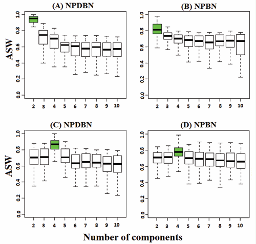
Figure 1 (A-B): – Comparative analyses between NPDBNs and NPBNs for the identification of the number of underlying cell-subpopulations. Datasets with a mixture of two subpopulations, sample proportion set to 1:1, number of proteins to 5, network density to 0.3, noise level to 0.5, and length of time series to 100. Boxplots show the results of the ASW. The ASW values are incomparable between different clustering approaches, but comparable between different parameters of the same method. The largest ASW value indicates the number of distinct subpopulations identified by the respective method. The outliers (dots) obtained from pooled values were left out. (C-D) –Same legend to (A-B) but for a mixture of four cell-subpopulations.

We employed a nonparametric measure, the average silhouette width (ASW), to provide a measure of how appropriately observations have been clustered (see definition in [15]). The use of this measure requires the fixation of the number of clusters in both methods. Therefore, an update of the number of components in the corresponding algorithm was eliminated, and the cluster number was set from 2 to 10 clusters. Consequently, we found both methods behave similarly in efficiency for the identification of the number of cell subpopulations in a cell-sample.

In Figure 2 and Figure 3 we evaluate the adequacy and stability of our NPDBN method as a function of variation of parameter levels such as the number of cell subpopulations, sample proportion, and intra-cell-subpopulation variability. As evaluation measure, we use the percentage of correctly allocated observations (pco) (see, e. g., [7]). In Figure 2, we observe that the accuracy in classification of observations decreases as the number of cell-subpopulations increases (Figure 2 A). On the other hand, a slight change in precision due to a variation in sample proportion is observed (Figure 2 B);

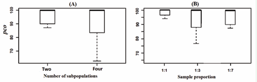
Figure 2: (A)-Boxplots of the percentages of correctly allocated observations (pco) using NPDBNs as a function of number of subpopulations. Datasets are from simulations with number of cell-subpopulations of two and four, sample proportion of 1:1, number of proteins of 5, network density of 0.3, noise level of 0.5, and length of time series of 100. Outliers obtained from pooled values were left out. (B)-Same legend to (A) but with sample proportion of 1:1, 1:3, 1:7, and mixtures of two cell-subpopulations.

however, there does not seem to be a direct relationship between the influence of the sample proportion and the adequacy of the model. In Figure 3, a comparative analysis of NPDBN is carried out with the static version NPBNs, in order to know how well our method classifies observations in presence of high levels of noise.

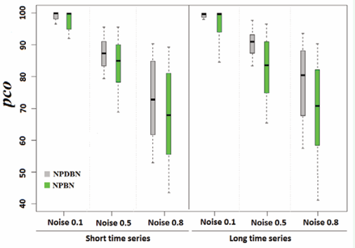
Figure 3: A comparative analysis between NPDBNs and NPBNs for different intra-cell-subpopulation variabilities. Boxplots show the pcos. Datasets are from simulations with two cell-subpopulations, sample proportion of 1:1, number of proteins of 5, network density of 0.3. Outliers obtained from pooled values were left out.

The NPBN method and its associated prior distributions were specified and implemented as in [7]. For all methods, the pco is directly affected by the noise level and slightly by the length of the size of the time series. A gradual increase is observed for the variation in its different noise levels. Here, the NPBNs present the bigger errors in the classification, which is due to the lack of inclusion of temporal correlations. This result demonstrates how the inclusion of temporal correlations can bring significant improvements in the classification of protein expression levels in time series. However, it is important to note that, although NPBNs do not allow the consideration of temporal correlations, they can classify the samples relatively well.

Figure 4 and Figure 5 contemplate a comparative evaluation of the network structures approximated with NPDBNs in terms of temporal conditional dependencies. To address this issue, we use ROC curves. A measure of precision is given by the area under the ROC (AUROC) curve. An area of 1 represents a perfect estimation, while an area of .5 represents a completely random estimation. For the above analyses, we know that some parameters, such as the number of nodes, network density, and intra-cell-subpopulation variability can affect the accuracy of our approach for the recognition of the true temporal protein interaction network. Here we found that the number of associated edges (Figure 4 A) can result in an increase of the mismatch of the model, while the number of nodes (Figure 4 B) is not a direct problem. On the other hand, the effect of the term intra-cell subpopulation variability is here also evaluated (Figure 4 C). As mentioned above, this term degrades the algorithm in terms of the amount of error increase.

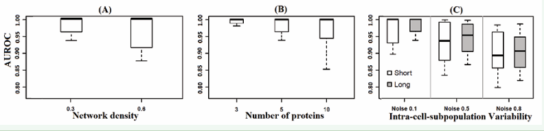
Figure 4: (A)-Boxplots of AUROC in function of network density. Datasets are from simulations with a mixture of two cell-subpopulations, sample proportion of 1:1, number of proteins of 5, network density of 0.3 and 0.6, noise level of 0.1, and length of time series of 100. The AUROC is used to compare how good the NPDBNs can recognize protein interaction networks. An area of 1 represents a perfect estimation, while an area of .5 represents an estimation based on randomness. Outliers obtained from pooled values were left out. (B) – Same legend to (A) but with number of proteins of 3, 5, and 10, and network density of 0.3. (C) – Same legend to (A) but with noise levels of 0.1, 0.5, 0.8, and length of time series of 20 and 100.

In Figure 5, a comparative analysis of the NPDBNs with NPBNs and with GDBNs is shown.

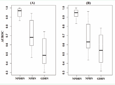
Figure 5: (A) - Boxplots containing the AUROC corresponding to the comparison of estimated and true protein interaction networks for the first cell-subpopulation in a mixture of two cell-subpopulations by using NPDBNs, NPBNs and GDBNs. Datasets are from simulations with mixtures of two subpopulations, sample proportion of 1:1, number of proteins of 5, network density of 0.3, noise level of 0.5, and length of time series of 100. Outliers obtained from pooled values were left out. (B)-Same legend to (A) but for the second cell-subpopulation.

NPBNs and GDBNs do not relate to each other, but nevertheless, present relevance in the analysis of protein interaction networks. Significant differences are observed when comparing the result of our approach with those obtained by the GDBNs without a previous classification of observations and the NPBNs without the inclusion of temporal correlations. In general, the use of GDBNs without a previous stratification of the data lead to mis-specified interaction models that do not resemble any of the true networks. The lack of adjustment presented in NPBNs is basically due to the non incorporation of associated edges to the same node known as a feedback loop. In this case, NPBNs tend to seek to compensate for this variation in another edge, thus moving away from the true structure. This is what leads to a decrease in accuracy.

CONCLUSION

Recent advances in the resolution of protein quantification techniques have led to the development of a methodology here called “Nonparametric Dynamic Bayesian Networks” for the incorporation of information from temporal relationships. Our work represents an improvement of the NPBNs [1] that were mainly developed to model static conditional dependencies by a directed acyclic graph for heterogeneous cell-populations. An optimal implementation of our method occurs by integrating out the parameters of the Gaussian conditional distribution given by Equation 5. The Nonparametric Bayesian Mixture Model here employed, provides a classification of the observations in homogeneous subgroups (or cell subpopulations). Each mixture component or cell subpopulation is characterized by a GDBN, where relationships between proteins are represented by a directed graph. These graphs contemplate the connections through directed edges, which are computed using Gaussian probability models (see Equation 6). The edges that represent the connections between the proteins are given by the algorithm in units of 0 and 1, where 1 means adjacency and 0 adjacent disconnection. A graph is estimated by the summary of the different adjacency matrices provided by the MCMC algorithm in [1]. A network structure, maximizing the posterior probability in Equation 7, is assigned to the computing component. The relations are of conditional dependence if non-adjacent proteins are conceded by means of a third protein, while the opposite leads to a conditional independence. Our analyses using synthetic protein interaction data in mixtures of two and four subpopulations, served to demonstrate by means of a comparison with the static version NPBNs and a single model provided by GDBNs the high suitability of our approach for the classification of observations and for the reconstruction of dynamic protein interaction networks even in the presence of high levels of noise.

ACKNOWLEDGEMENTS

We would like to thank Dr. Eli Zamir, Max Planck Institute for Medical Research, Heidelberg, Germany, and Dr. Hernán E. Grecco, Universidad de Buenos Aires, Argentina, two coauthors from articles as [1] and [7], for valuable contributions to this manuscript. Yessica Fermin would also like to thank the German Academic Exchange Service DAAD and the TU Dortmund University for their financial support.