This study examines infant mortality, a critical global health issue, particularly in developing countries with economic disparities affecting healthcare access. It compares the forecasting accuracy of three econometric models Vector Error Correction Model (VECM), Vector Autoregressive (VAR), and Bayesian VAR (BVAR), to predict infant mortality rates (IMR). The analysis uses data on IMR, neonatal mortality rates (NMR), and Ugandan GDP and GDP per capita (GDPP), from 1954 to 2016, assessing model performance through statistical measures like Mean Squared Error (MSE) and Theil’s U-statistic.

The results reveal significant long-term relationships between IMR, NMR, GDP, and GDPP, with VECM being the most accurate model for long-term forecasting, achieving an adjusted R-squared of 97.7%. Impulse response analysis shows GDP positively impacts IMR, while GDPP has a stronger long-term effect in reducing IMR. For NMR, GDP has a negative effect, while GDPP shows a positive response over time. Granger causality tests confirm bidirectional causality between GDPP and IMR, while IMR unidirectionally influences GDP. Projections indicate Uganda’s IMR could decline to 17 deaths per 1,000 live births by 2035, although the decline in NMR will slow.

In conclusion, short-term forecasts are best modeled by ARIMA, while long-term forecasts are more accurately captured by VECM. GDPP has a more substantial impact on reducing IMR and NMR than GDP, highlighting the importance of equitable resource distribution and macroeconomic growth for improving child survival rates.

• Infant Mortality Rate; Neonatal Mortality Rate; Vector Error Correction Model; Gross Domestic Product per Capita; Time Series Analysis

Odur B, Etil T, Opio B, Memon S (2025) Comparing Forecasting Models for Predicting Infant Mortality: VECM vs VAR and BVAR Specifica- tions. Pediatr Child Health 13(2): 1352.

Infant mortality remains one of the most critical health challenges worldwide, particularly in developing regions such as Sub-Saharan Africa. Despite significant global progress in reducing mortality rates over the past few decades, millions of children continue to die before their fifth birthday, with infant mortality (IMR), and neonatal mortality (NMR), accounting for a large proportion of these deaths. In 2019 alone, more than 5 million children under the age of five died, and the global decline in mortality has been slower for neonatal deaths compared to post-neonatal deaths (Sharrow et al., 2022). This disproportionate loss of young lives is often attributed to preventable or treatable causes such as neonatal encephalopathy, infections, complications due to preterm birth, and malnutrition [1]. For example, neonatal mortality, which refers to deaths in the first 28 days of life, has been a major focus of global health policy, especially in low-income countries where healthcare access and infrastructure are limited [2].

In countries like Uganda, infant and neonatal mortality rates remain a major concern despite efforts to improve healthcare access. Factors such as maternal education, per capita income, health expenditure, and environmental conditions are critical determinants of infant health outcomes [3]. However, despite interventions aimed at improving healthcare delivery and access to essential services like mosquito nets and oral rehydration therapy, infant and neonatal mortality rates in Uganda remain high compared to regional peers. As a result, there is a significant gap in understanding how macroeconomic factors such as GDP per capita and GDP can best be used to forecast the future infant and neonatal mortality rates. Several studies have also examined the impact of economic conditions on infant and maternal mortality. Ensor et al. [4], studied the effect of GDP fluctuations on maternal and infant mortality, finding a negative correlation during economic recessions, particularly in developing nations. Their findings emphasized the significant role of economic growth and health system performance in shaping health outcomes, particularly in low-income countries.

In this context, examining how these factors interrelate with mortality rates becomes essential for designing effective policies aimed at achieving the SDG target of reducing under-five mortality to 25 per 1,000 live births by 2030 [5]. The causal effect of maternal and child mortality on GDP is generally stronger in HICs and UMICs due to the differences between poor and rich countries with respect to the human capital level or infrastructure. Human capital is the stock of competencies, knowledge, and social and personality attributes, including creativity, embodied in the ability to perform labor so as to produce economic value. The higher human capital level of richer countries compared to poorer countries implies that an equal reduction in maternal and child mortality will cause GDP to increase more in richer countries than in poorer countries [6].

Erdil et al. [7], applied the Granger-causality approach to a panel data model with fixed coefficients in order to determine the relation between GDP and health expenditures per capita. They found significant bidirectional causality even for such a short time period, signaling that the evidence may be stronger for longer time periods. However, this causality is not homogenous, which is evident from the tests of the HC hypotheses. For one- way causality, the pattern of causality is different in low- and middle-income countries as compared to high-income countries. One-way causality generally runs from GDP to H in LIC and MIC, whereas the reverse holds for HIC.

Forecasting Models in Health Economics

The application of econometric models to forecast health outcomes, such as infant mortality rates (IMR), and neonatal mortality rates (NMR), has gained significant attention in recent years. These models help to capture the complex interactions between various socioeconomic and macroeconomic factors affecting health outcomes. Among the most widely used econometric techniques are Vector Error Correction Models (VECM), Vector Autoregressive (VAR) models, and Bayesian VAR (BVAR) specifications. Each of these models offers unique strengths, particularly in their ability to account for dynamic relationships between variables, their ability to model both short- and long-run effects, and their robustness in the face of uncertainty.

Recent research has applied various forecasting models to predict Infant Mortality Rates (IMR), and Neonatal Mortality Rates (NMR). In India, a study by Mishra, Sahanaa, and Manikandan (2019) utilized ARIMA models to forecast IMR from 1971 to 2016. The ARIMA (2, 1, 1) model demonstrated high forecast accuracy, with projections showing a decline in IMR from 2017 to 2025, predicting an IMR of 15 per 1,000 live births by 2025. Khan et al. (2019) conducted a similar analysis for Asian countries using log- log regression and ARIMA models. Their study found a strong correlation between IMR and GDP per capita, with ARIMA (AR(1)) models effectively forecasting IMR from 1980 to 2015, with forecasts extending to 2025.

In Nigeria, Usman et al.[8], applied ARIMA models to analyze newborn mortality trends, revealing a significant decline from 51.7% in 1990 to 33.9% in 2017. The ARIMA (1, 1, 1), model was found to provide the best fit for this data. Similarly, Ogedi et al. [9], compared ARIMA with other time series methods such as Simple Exponential Smoothing (SES) and Brown’s Linear Trend (BLT), using Bayesian Information Criterion (BIC) to evaluate model adequacy. They concluded that the ARIMA (0, 2, 0) model was the most suitable for forecasting NMR in Nigeria, outperforming other models based on Theil’s U and MAPE metrics.

Kurniasih et al. [10], evaluated the forecasting accuracy of ARIMA, Holt-Winters, and the α-Sutte Indicator for mortality rates. Their analysis revealed that the α-Sutte Indicator outperformed both ARIMA and Holt-Winters, with lower Mean Squared Error (MSE) and Mean Absolute Percentage Error (MAPE), suggesting its superior predictive ability. Bhowmik [11], explored the relationship between GDP, health expenditure, and the Human Development Index (HDI) in the SAARC region. Their panel data analysis identified long-term causal links between GDP and health spending to HDI, with no immediate causal effects, highlighting the role of sustained health investment in improving human development over time.

Vector Error Correction Models (VECM)

The Vector Error Correction Model (VECM), is a powerful econometric tool designed to examine long- term relationships between non-stationary time series data, such as macroeconomic indicators and health outcomes. VECM is particularly effective when variables are cointegrated, meaning they share a stable long-term equilibrium. In the context of infant mortality, VECM is valuable for analyzing how factors like GDP per capita and GDP impact Infant Mortality Rates (IMR), and Neonatal Mortality Rates (NMR) both in the short and long run. This model is widely used across various fields, including health economics. For example, Lin and Lee [12], applied VECM to explore the relationship between healthcare spending and life expectancy, revealing strong long-run connections between economic factors and health outcomes. Similarly, in the case of infant mortality, VECM helps uncover how improvements in socioeconomic variables, such as income contribute to the sustained reduction of mortality rates over time [13].

Zhou et al. [14], used VECM to model mortality rates, finding that the model was effective in identifying long-term equilibrium relationships among key variables. Similarly, Arnold and Sherris [15], applied VECM to assess cause- of-death mortality rates, demonstrating its capability to capture long-term dependencies and enhance forecasting accuracy compared to traditional ARIMA models. In Greece, Siahanidou et al. [16], used VECM to analyze IMR trends from 2004 to 2016, revealing that socioeconomic factors such as the Human Development Index (HDI) and rural residency significantly influenced IMR.

Vector Autoregressive (VAR) Models

The Vector Autoregressive (VAR) model is another econometric tool frequently used in health forecasting, particularly for analyzing the interdependencies between multiple variables without assuming a specific causal relationship. Unlike VECM, which focuses on cointegration, VAR models are useful for exploring how changes in one variable affect other variables in the system over time. This makes VAR particularly useful when the researcher wants to understand how different macroeconomic variables such as GDP and GDP per capita affect IMR and NMR.

Liao et al. [17], used VAR models to analyze the relationship between health expenditures and health outcomes in China, showing that both healthcare spending and economic growth are significantly related to life expectancy and infant survival. Similarly, Imo et al., applied VAR to investigate the causal relationships between economic growth, public health investments, and IMR in sub-Saharan Africa. Their findings suggested that while short-run variations in health outcomes are driven by healthcare investments, long-term improvements in IMR require broader economic growth and socioeconomic development.

Faye et al. [18], applied a Vector Autoregressive (VAR), model to assess the relationship between health expenditure, GDP, and IMR in the Philippines. Their results showed that health expenditure had a significant impact on IMR, whereas GDP per capita was more influential in reducing under-five mortality rates. In a similar vein, Shannon R. Lane [19], explored the impact of public health expenditure on national health outcomes, observing a negative correlation between government health spending and IMR, indicating that increased public health investment can reduce infant mortality. Chung and Muntaner [20], investigated the impact of income inequality on infant mortality across various countries. They found that public health services were the only consistent factor linked to reduce IMR, whereas income inequality did not have a direct effect on health outcomes. Therefore, VAR models are well-suited to forecast how changes in key variables will influence future trends in infant and neonatal mortality, particularly when short-run dynamics and the feedback effects between variables are of interest.

Bayesian VAR (BVAR) Models

Bayesian Vector Autoregressive (BVAR), models are an extension of traditional VAR models, integrating Bayesian statistical methods to handle uncertainty and improve estimation accuracy, especially when data is limited or noisy. A significant advantage of BVAR is its ability to incorporate prior knowledge or external information, leading to more robust forecasts, particularly when working with small datasets or when prior insights into the relationships between variables are available.

BVAR models have gained increasing popularity in forecasting applications, particularly in health outcomes. For instance, Kholid et al. [21], used BVAR to forecast health outcomes in low-income countries, demonstrating its capacity to deliver more accurate predictions despite limited data. In the context of infant mortality, BVAR is particularly valuable for forecasting long-term trends, as it allows for the inclusion of prior knowledge regarding the influence of factors like maternal education, sanitation, and healthcare spending. Additionally, the flexibility of BVAR models makes them ideal for addressing the uncertainty inherent in predicting future health trends, offering significant advantages for policy-making in resource- constrained settings [22].

BVAR models have been proven to improve forecast accuracy by accounting for parameter uncertainty. Guibert, Lopez, and Piette [23], underscored the importance of decomposing mortality rates into latent components and suggested that BVAR is particularly suited for long-term mortality rate projections. In Australia, studies found that BVAR models outperformed traditional VAR models in terms of forecast accuracy, with the incorporation of parameter risk being a crucial factor [10].

Njenga [24], highlighted the flexibility of VAR models in capturing trends and correlations in mortality data. By integrating Bayesian techniques, BVAR models can provide more reliable forecasts, as demonstrated in Australian mortality rate studies that compared out-of- sample predictions from both BVAR and traditional VAR models [15].

Comparison of VECM, VAR, and BVAR Models

Although VECM, VAR, and BVAR models are widely used in health forecasting, there is a lack of comprehensive studies comparing their effectiveness in predicting infant and neonatal mortality rates. Fernández et al. [25], compared the performance of VAR and BVAR models in forecasting macroeconomic variables and found that BVAR models provided more accurate predictions, especially when uncertainty was present. Similarly, Dube et al. examined the use of VECM and VAR in forecasting health outcomes in developing countries. They concluded that VECM was more effective at capturing long-term relationships, while VAR models provided better short- term forecasts.

The comparison of these models is vital for identifying the most accurate and reliable tool for forecasting Infant Mortality Rates (IMR), and Neonatal Mortality Rates (NMR), in both short and long run, considering the dynamic nature of health systems and the complex relationships between macroeconomic factors. Understanding how these models perform is particularly important as countries work toward meeting the SDG targets for child health. Accurate forecasting is essential for informing policy decisions related to resource allocation, healthcare interventions, and long-term planning aimed at achieving these targets. This article offers a detailed comparison of VECM, VAR, and BVAR models, focusing on their ability to predict future trends in infant mortality based on historical data and macroeconomic variables. It also contributes to the growing body of literature on the intersection of economics, health outcomes, and forecasting techniques.

Data Sources

The study utilized country-specific annual infant and neonatal mortality rates data compiled and provided by http://www.childmortality.org. UN IGME web site data used in the United Nations Children’s Fund (UNICEF) Report on levels and trends in Child Mortality. Data on Ugandan GDP and GDP per capita was obtained from the World Bank web site. The researchers used GDP at 2000 US prices (the World Bank’s World Development Indicators 2016; http://devdata.worldbank.org/wdi2016.htm).

Procedures

The projection of infant and neonatal mortality based on the vector error correction model from 2030 was done using time series data from 1954 to 2016, collected from UNICEF, the Bank of Uganda, the Ministry of Water and Environment, and the Ministry of Finance Planning and Economic Development. Variables considered here include: infant mortality rate, neonatal mortality rate, country’s GDP per capita, and GDP.

Forecasting the infant and neonatal mortality

Three stages of analysis were adopted to facilitate the achievement of the goal. In the first stage, the study examined the trends and patterns of infant and neonatal mortality rates, government health expenditure, GDP, GDP per capita, sanitation coverage, and maternal literacy levels. The study was further focused by conducting an optimal lag length determination and a co-integration test. The second stage involved time series analysis (VAR, BVAR, and VECM) in order to determine the relationships and effects of the aforementioned variables on health outcomes. Lastly, the study devoted stage three to performing an out-of-sample projection of infant and neonatal mortality rates in 2030.

Time series analysis was used to identify the magnitude and direction of the relationship between health outcomes and GDP, GDP per capita, government health expenditure, sanitation coverage, and maternal literacy.

Statistical Analysis

Trend and patterns of infant and neonatal mortality rates, Ugandan GDP, GDP per capita were explored through graphs

Stationarity assessment of the variables

All the series (IMR, NMR, GDP, and GDPP) were tested for stationarity before they were fixed into the model. According to Granger and Newbold (1974), if there is a unit root, then that particular series is considered non- stationary.

A stochastic time series Yt is said to be stationary, if and only if, it satisfies the following assumptions:

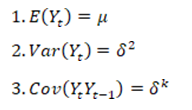
Conditions (1) and (2) imply that has a constant mean and variance over time, while condition (3) means that the covariance between series depends only on how far apart they are and not on the time of occurrence (Danao [26,27]. If one or more of the above conditions are not satisfied, the series is non-stationary, and proceeding with regression analysis would result in spurious results, which can produce high t-statistics but have no coherent economic meaning or an insignificant result.

Dicky Fuller Unit Root test for stationarity in the series

The Augmented Dicky-Fuller (ADF) standard test for unit root in the series was used in testing for the presence of unit root in both transformed and non-transformed series. The time series data in this study can take any of the following stationarity models:

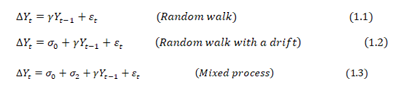
The error terms e are assumed to be independent and identically distributed. Dickey and Fuller [28], proposed the ADF test in order to handle the autoregressive process in the variables [28]. Where the ADF indicated the occurrence of a unit root, then the series is non-stationary In case of non-stationary, then the researcher proceeded to taking the logarithms, differencing until he arrive at a stationary series.

Many scholars used differencing to detrend the data and control autocorrelation by subtracting each datum in a series from its predecessor until stationarity was attained (Deluna, 2014). Once stationarity is attained after differencing d times, the series is said to be integrated in order d [26]. In such cases, the researcher then proceeded with optimum lag length determination and co-integration analysis.

Model Specification and Identification

The first step in building a VAR (p) model involved model identification. This helps in identifying the appropriate model’s order. The most common methods used for lag order determination include Akaike Information Criterion (AIC) [27], Schwarz-Bayesian (BIC), and Hannan-Quinn (HQC). The main idea of AIC is to select the model that minimizes the negative likelihood penalized by the number of parameters.

The AIC and SBC equations are given below:

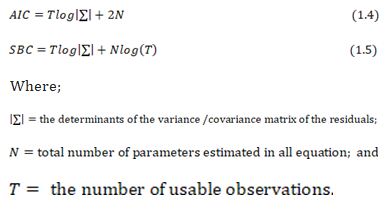
Both AIC and SBC differ in their exact definition of a good model. In this case, the study choose the model which has the lowest AIC and SBC values.

The time series Yt, where

 denote an (n×1) vector variables, follows a  model if it satisfies 

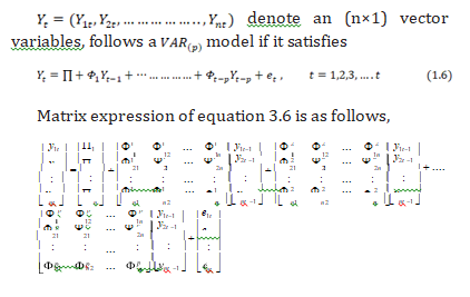
Where P is a k-dimensional vector, F1 , F 2 ,…….,

F p are k*k parameter matrices and et is a sequence of

independently and identically distributed error vector.

Assumptions of the errors: -

The error term et is a multivariate normal k * 1 vector of error satisfying the following assumptions;

1. E ( et )=0 every error term has mean zero;

E (e e' ) = s the contemporaneous covariance matrix of error terms is w (a n*n positive semi-definite matrix);

1. E (e e'    ) = 0 for any non-zero k. There is no correlation across time; in particular, no serial correlation in individual error terms and F j are k*k matrices.

   Lag length determination

2. Four basic variants of the model were estimated:

3. the VEC model using both the Chao and Phillips (1999) joint procedure, VEC(J), and the more standard sequential procedure based on using the BIC to select the lag length and Johansen and Juselius’s (1990) maximum root test to select the number of common trends using a sequence of 5% tests, VEC(S).

4. a VAR using BIC to select the lag length.
5. a DVAR using BIC to select the lag length.
6. Two BVARs, each using AIC to select the lag length, but with either the standard Minnesota priors (with hyper parameters of 0.2 for the diagonal and 0.2 for the off- diagonal terms), BVAR (M), or with looser priors on theoff-diagonal (off-diagonal hyper parameter = 0.8), BVAR (L).
   Vector Autoregressive Processes
   According to Sims [29] and Litterman (1976, 1986), Vector Autoregressive (VAR), models have been proven to forecast better than any simultaneous equation models. Vector Autoregressive (VAR), models provide information about a variable’s forecasting ability for another variable. It is an econometric model used to capture the evolution and the interdependence between multiple time series. In order to build a VAR model [27], certain steps can be followed. This includes model identification, estimation of constants, a diagnostic check, and finally forecasting. Conditional heteroscedasticity and outliers in the residual series are also checked. The existence of co-integration was used to check for the presence of any common trends, and finally, an Error Correction Model (ECM), was developed due to presence of co integration to improve the long-term forecast.

7. Estimation of the VAR model

   After obtaining the order of the model, p, of the vector series, the researcher derived the estimators of the constants as in the steps below.

   Consider the consecutive VAR models:
   

   The most common methods of estimating parameters are the maximum likelihood estimator (MLE) and the ordinary least square estimator (Yang & Yuan, 1991). Here, the study applied the ordinary least squares (OLS), method to estimate the parameters of these models and apply equation by equation.

   For  equation (7), let  be the OLS estimate of and  be the OLS estimate of . Where (i) is used to denote the estimate of a VAR (i) model. The estimates of the coefficients of the VAR model.

    When estimated using unrestricted VAR (p) model are considered to be fixed quantities. These estimates of coefficients do not accurately reflect the underlying relationship because some of the estimated coefficients of the VAR model are non-zero purely by chance when estimated by OLS so restrictions may be imposed to reduce the number of parameters being estimated, Mercy et al., (2015).

   Diagnostic Check for VAR model

   Suppose the orders and constants have been chosen for a VAR model underlying the data, then residuals are checked to see whether they are normally, identically, and independently distributed. After the model had been fitted, heteroscedasticity was tested through multivariate arch tests; autocorrelation through Durbin Watson; normality through Jarque-Bera tests; the unit root test through the Dickey Fuller and Augment Dickey Fuller tests; and the statistical significance of the parameters was tested through t statistics. For details, look at Mercy et al., (2015).

   Data Description

   Standard practice in VAR analysis is to report results from Granger causality tests, impulse responses, and forecast error variance decompositions. These statistics are computed automatically (or nearly so), by many econometrics’ packages. Because of the complicated dynamics in the VAR, these statistics are more informative than the estimated VAR regression coefficients or statistics, which typically go unreported. Granger-causality statistics examine whether lagged values of one variable help to predict another variable.

   Bi-variate Granger causality was used to determine which national variables help predict health outcomes. If a variable Granger causes a health outcome, it is included in the VAR and BVAR forecasting models. These tests were conducted for each health outcome at lag length 1,2,3,4 and 5 years using both a deterministic time trend and first differences.

   Forecasting models

   Bayesian Vector Autoregressive (BVAR) was used in this study to assess whether prior information on spatial and economic base-sectoral linkages improves forecast accuracy for health outcomes in Uganda. The study then forecasted the mortality levels using VAR and BVAR models to compare their forecasting accuracy.

   Assessment of forecast performance or VAR and BVAR

   Alkema and New (2012), concluded that, point estimates on child mortality based on limited information may substantially under- or overestimate the truth. Uncertainty assessments can and should be used to complement point estimates to avoid unwarranted conclusions about levels or trends in child mortality and to reduce confusion about differences in estimates within and between countries. In this study, both bootstrapping and cross-validation were used to assess the predictive power of the models, and the best model was used to project the infant and neonatal mortality by 2030 or 2035.

   Infant and neonatal mortality forecasts

   Time series analysis uses the factor of time to replace other kinds of influencing factors. Li Y, et al. (2017) used the autoregressive integrated moving average (ARIMA) model, one of the classic methods of time series analysis based on past values of a series and previous errors, to forecast under-five mortality in India. Despite all the advantages of this approach, it does not consider the influence of other macro variables in the economy like the Vector Auto Regressive model. The study then considered the infant and neonatal mortality rates from 1954 to 2014 as a training sample to fit the VAR model, and 2015–2017 was considered for the within and without samples for internal and external validation, respectively.

   To compare the performance of the VECM, VAR and BVAR models, the researcher computed the mean square error, root mean square error, and Theil’s U statistics for the quality of the time series forecast methods.

For a  model, the 1-step ahead forecast at the tim e origin h is given by;

The associated forecast error is

The covariance matrix of the forecast error is Σ. If Yt is weakly stationary, then 1-step ahead forecast Y1(1) converges to its mean vector, µ, as the forecast horizon increases, Mercy et al., 2014.

Mean Squared Error (MSE): Any of the two models was considered best if it has the minimum forecast error arising from comparing the actual value and forecast value.

Root Mean Squared Error (RMSE) Is the square root of the average of all squared errors, according to Wang and Lim (2005). It ignores any over and under- estimation.

Theil’s U Statistic: Theil’s U-statistics see Theil (1958) is used as a measure of forecasting error that is minimized. It is a relative measurement based on comparison of the predicted change with the observed change. The value of U lies between 0 and 1. If U equals to 0, there is a perfect fit, whereas U equals to 1 implies that forecasting of data is very poor.

Assessment of the forecasting accuracy of BVAR, VECM and VAR model

However, the forecast of infant mortality from 2030 forward is very important in knowing what infant and neonatal mortality would look like if nothing is done to address the risks of infant and neonatal mortality. This paper provides exploratory results on the forecasting powers of three econometric models such as BVAR, VECM, and VAR in estimating the future IMR and NMR in Uganda based on historical data.

The distribution of IMR, NMR, health expenditures, GDP per capita, GDP, Sanitation cover and maternal literacy cover

Here, the distribution and stationarity of eight selected study variables, which included infant mortality rate (IMR), neonatal mortality rate (NMR), Ugandan GDP (GDP), GDP per capita (GDPP) were performed. Whereas a visual trend of selected variables was done through graphs, statistical tests for stationarity using the Augmented Dicky-Fuller Unit Root Test at 5% were equally done. Where variables displayed unit root (non-stationarity), they were converted to stationarity by taking the logarithm and differencing until stationarity was achieved.

Lag length for modelling IMR

The maximum lag length of five (5) was chosen based on the lowest value of AIC, FPE, LR, and HQIC to model IMR (Table 1).

Table 1: Lag length determination based on AIC (IMR)

lag	LL	LR	Df	P	FPE	AIC	HQIC	SBIC
0	-1790.50				1.4e25	66.4261	66.4687	66.5366
1	-1515.161	549.40	9	0.000	7.5e20	56.5854	56.7558	57.0274
2	-1452.13	127.34	9	0.000	1.0e20	54.5605	54.8588	55.3340*
3	-1440.62	23.04	9	0.006	9.2e19	54.4673	54.8934	55.5722
4	-1429.19	22.86	9	0.007	8.5e19	54.3773	54.9313	55.16138
5	-1413.25	31.87*	9	0.000	6.8e19*	54.1204*	54.8023*	55.16884

Define *

Similarly, a maximum lag length of four (4) was determined based on the same approach to model NMR in Uganda (Table 2).

Table 2: The Lag length determination based on AIC (NMR)

lag	LL	LR	Df	P	FPE	AIC	HQIC	SBIC
0	-1599.32				5.1e24	65.4008	65.4448	65.5167
1	-1329.12	540.40	9	0.000	1.2e20	54.7396	54.9154	55.2029
2	-1269.35	119.55	9	0.000	1.5e19	52.6672	52.9748	53.4780
3	-1228.92	80.845	9	0.000	4.2e18	51.3846	51.8241	52.5429*
4	-1214.50	28.853*	9	0.001	3.5e18*	51.1631*	51.7344*	52.6689
5	-1211.57	5.16459	9	0.755	4.6e18	51.4112	52.1143	53.2644

Determination of the direction and magnitude of the relationships between health outcomes and macroeconomic variables

Given that the study focused on two health outcomes (IMR and NMR), we selected the appropriate model for assessing the relationship between health outcomes and independent variables.

Choice of model

Chepngetich and John (2015), reported that VAR models are used to describe and forecast multivariate time series for stationary time series and recommended that for 

non-stationary time series, a vector error correction term is added to form a vector error correction model (VECM). It was therefore necessary to test for the existence of a stationary linear combination of the non-stationary terms (co-integration). I transformed the selected series into a vector error correction model (VECM) by taking the first difference, which in turn facilitated long-term forecasting. Those series that were not stationary at the first difference were dropped from the forecasting model.

Vector Auto Regressive model to assess the relationship between IMR and GDP, GDPP

Understanding how the variables relate to changes in the outcome variables is important in planning and policy formulation. As a result, I investigated the relationship between LIMR, LNMR, LGDP, and LGDPP.

Impulse Response

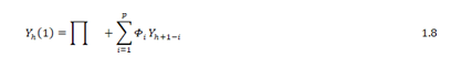
The first step taken in building a VAR (p) model was the identification of the appropriate model (lag length), using the Akaike Information Criterion (AIC). The main idea of AIC is to select the model that minimizes the negative likelihood penalized by the number of parameters. The VAR model was then fitted to investigate how changes in the independent variables (LGDP and LGDPP) could affect the health outcomes (LIMR and LNMR) as presented in Figure 1.

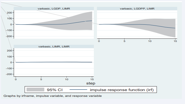
Figure 1: Impulse response function for infant mortality rates to shocks in GDP, GDPP and NMR

The response of LIMR to a one standard deviation (SD) shock (innovation) in LGDP remained steady at about zero in the first five years and increased slightly in the subsequent five years; however, beyond 10 years, LIMR rose above average quickly as compared to the previous period and it remains in the positive region. That is, shocks to LGDP will have a positive impact on LIMR in both the short and long run. Furthermore, the effect of a one SD shock in the LGDPP was not noticeable in the short run and declined in the negative region slowly in the period between five and ten years, but it decreased rapidly beyond 10 years. This implied that the shock to LDGPP will have a negative impact on LIMR in the long run; that is, an increase in a country’s GDPP leads to an increase in health infrastructure development in the long run, which in turn leads to a drop in infant mortality (Figure 1). Impulse response of NMR to a one SD shock on LGDP and LGDPP

The response of LNMR to a one SD shock (innovation) on LGDP was about zero in the first three years, and it decreased rapidly between three and ten years; it remained steadily between 10 and twelve years. Beyond twelve years, LNMR registered a quick rise but remained in the negative region. In other words, a one SD shock in LGDP has a negative impact on LNMR in both the short and long run (Figure 2).

Figure 2: Impulse response function for infant mortality rates to shocks in GDP, GDPP and IMR

Similarly, while the impact of a one-SD shock in LGDPP on LNMR was not noticeable in the period zero to five years, the response rapidly increased between the five- and ten-year periods, where it hit a steady value for about two years. The response of LNMR to stimulation in LGDPP started declining but remained in the positive region beyond 12 years. This meant that a shock to LGDPP would benefit LNMR in both the short and long run (Figure 2).

Engle Granger Causality GDP and GDPP on Health outcome (IMR and NMR)

Based on variables such as IMR, GDP, and GDPP, it was noted that GDPP significantly influences IMR in the short run. In addition, Uganda’s GDP and GDPP all together cause changes in IMR in the short run. In a similar twist, it was discovered that IMR causes GDP, yet GDPP was found not to be significant in causing GDP. It’s worth noting that both IMR and GDPP influence a country’s GDP. It was also observed that IMR significantly causes GDPP and that there were no significant causal effects between GDP and GDPP (Table 3).

Table 3: Test of granger causality among IMR, NMR, GDP and GDPP

Equation	Excluded	x2	Df	P value
LNMR	LGDP	35039	3	<0.001*
LNMR	LGDPP	1.4e5	4	<0.001*
LNMR	ALL	9.7	7	<0.001*
LGDP	LNMR	5.4705	4	0.242
LGDP	LGDPP	5.7e6	4	<0.001
LGDP	ALL	6.0e6	8	<0.00
LGDPP	LNMR	5.487	4	0.241
LGDPP	LGDP	1.4e6	3	<0.001*
LGDPP	ALL	2.0e7	7	<0.001*
LIMR	LGDP	1.2e7	5	<0.001*
LIMR	LGDPP	8.6e6	3	<0.001*
LIMR	ALL	1.8e8	8	<0.001*
LGDP	LNMR	13.733	5	0.017
LGDP	LGDPP	3.9e5	3	0.001*
LGDP	ALL	8.3e5	8	<0.001*
LGDPP	LNMR	13.754	5	0.017*
LGDPP	LGDP	9.9e5	5	0.001*
LGDPP	ALL	1.0e6	10	0.001*

*Significant variable at 5%

The findings revealed a significant two-way causality between IMR and GDPP and a one-way causal effect from IMR to GDP. Interestingly, it was clear that GDP only causes IMR through GDPP. There was no causality between GDP and GDPP in the short term. In view of the above, four variables that caused an increased infant or neonatal mortality rate were included in the VAR, VECM, and BVAR models.

There was a strong relationship between health outcomes (such as IMR and NMR) and GDP, just like GDPP, which could be due to the level of human capital dependency and the higher marginal effect of health spending on LIC and LMIC. This was in agreement with the research conducted by Amiria and Gerdtham [6], who found that there was a stronger relationship because the effects of GDP on health are stronger in LIC and LMIC compared to HIC and UMIC, while in contrast, the effects of health on GDP are stronger in HIC and UMIC compared to LIC and LMIC. The tests were run with a lag length of four for neonatal mortality and five for infant mortality as predetermined in lag length selection procedures (Table 3).

The Granger causality test was employed to determine whether lagged values of GDP (LGDP), and GDP per capita (GDPP), could predict infant mortality rate (LIMR), and neonatal mortality rate (LNMR). The findings indicate a strong causal relationship, as the lagged values of both LGDP and GDPP significantly influence LIMR, with p-values less than 0.001. This suggests that changes in GDP and GDPP can effectively predict future infant mortality rates in the short term. Furthermore, a direct causal effect of LGDP and GDPP on LNMR was also observed, confirming that these variables are useful for forecasting neonatal mortality rates. However, the lagged values of LNMR did not independently affect LGDP, but they did show a significant effect when combined with LGDPP (p = 0.017). Similarly, LIMR did not exhibit a direct causal effect on GDPP alone, but this relationship became significant when considering the interaction with LGDP. Overall, while LNMR has a significant influence on both LGDP and GDPP, the direct causal relationships among these variables highlight the complex interdependencies in predicting mortality rates in the context of economic factors (Table 3).

Johansen Cointegration Test

IMR, NMR, GDP, and GDPP were among the variables taken into account in this study. They were non-stationary at level but became stationary after the first difference. Based on these results, I used the Johansen test of co- integration at 5% to check for co-integration. This assisted in determining whether the variables move together over time or not, which in turn assisted in choosing between fitting the VAR model and the VECM. Results revealed that there was an order 1 co-integration between LIMR, LGDP, and LGDPP, as well as an order 2 co-integration between LNMR, LGDP, and LGDPP. This meant that these three variables move together in the long run, hence the need to fit the Vector Error Correction Model (VECM) for both NMR and IMR.

Assessment of the forecasting performance of VECM and BVAR

To keep things simple, the analysis results showed that there was co-integration of order one for infant mortality data (IMR) and order two for neonatal mortality data (NMR). The study considered the first order of co- integration in the subsequent analysis. With the presence of co-integration in the data set, VECM was found to be more appropriate for making long-term projections than the VAR model, whose supremacies were observed only in the short run. However, there was a need to compare the projection accuracy between VECM and BVAR (Table 4).

Table 4: Assessment of the infant mortality rate projection accuracy

Variable	Inc. obs.	RMSE	MAE	MAPE	Theil
BVAR	8	0.067645	0.050364	1.441729	0.009243
VECM	8	0.010883	0.009870	0.269412	0.001475

RMSE: Root Mean Square Error

MAE: Mean Absolute Error

MAPE: Mean Absolute Percentage Error

Theil: Theil inequality coefficient

To accomplish this, the dataset was divided into two parts (the training data was sampled from 1954 to 2010, and the validation data was sampled from 2011 to 2018). The accuracy levels for within-sample forecasts were assessed using Root Mean Squared Error (RMSE), Mean Absolute Error (MAE), Mean Absolute Percent Error (MAPE), and the Theil Inequality Coefficient. In all cases, the model with the minimum possible errors was taken to be the best (Table 4).

The results in Table 4 revealed that, in the long run, the model that can best predict infant mortality rate in Uganda is VECM since it has smaller values of the projection errors as compared to BVAR.

Table 5 indicates that the Vector Error Correction Model (VECM),

Table 5: Assessment of the neonatal mortality rate projection accuracy

Variable	Inc. obs.	RMSE	MAE	MAPE	Theil
BVAR	8	0.065402	0.047626	1.405643	0.009164
VECM	8	0.00864	0.007132	0.233326	0.001396

RMSE: Root Mean Square Error MAE: Mean Absolute Error

MAPE: Mean Absolute Percentage Error Theil: Theil inequality coefficient

demonstrated superior accuracy in projecting neonatal mortality rates, as evidenced by its lower forecast error values compared to the Bayesian Vector Autoregression (BVAR) model. Consequently, VECM was selected for forecasting infant and neonatal mortality rates from 2021 to 2035. The study further explored the relationships among Infant Mortality Rate (IMR), Neonatal Mortality Rate (NMR), Gross Domestic Product (GDP), and GDP per capita (GDPP), to assess the impact of changes in GDP and GDPP on IMR and NMR. To quantify this effect, forecast error variance decomposition was employed, measuring the extent to which variations in GDP and GDPP account for changes in IMR and NMR over both short and long-time horizons.

Infant mortality rate in VECM

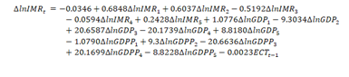
Based on the long run equation, it was clear that LGDP has a negative effect on IMR whereas GDPP has a positive effect on infant mortality, and the coefficients were significant at the 5% level. In a nutshell, LGDP and LGDPP have a symmetric effect on LIMR in the long run, on average, ceteris paribus. Overall, the VECM fitted the data very well, with an adjusted R squared of 97.7%. Further still, the F-statistics were significant at the 1% level (Table 6).

Table 6: VECM with LIMR as the dependent variable (Data 1954-2018)

Variables	Coef.	Std. Err.	Z	p-value
ECT
L1.	-0.002339	0.000943	-2.480684	0.018*
LIMR
LD.	0.684889	0.164376	4.166600	<0.001*
L2D.	0.603716	0.213071	2.833400	0.008*
L3D.	-0.519278	0.211802	-2.451716	0.019*
L4D.	-0.059496	0.245058	-0.242785	0.809
L5D.	0.242812	0.190733	1.273047	0.211
LGDP
LD.	1.077618	5.481750	0.196583	0.845
L2D.	-9.303459	17.02088	-0.546591	0.588
L3D.	20.65873	23.54561	0.877392	0.386
L4D.	-20.17390	17.17973	-1.174285	0.248
L5D.	8.818011	5.635692	1.564672	0.126
LGDPP
LD.	-1.079008	5.481226	-0.196855	0.845
L2D.	9.300009	17.02017	0.546411	0.588
L3D.	-20.66295	23.54524	-0.877585	0.386
L4D.	20.16990	17.17955	1.174064	0.248
L5D.	-8.822784	5.636068	-1.565415	0.126
_Cons	-0.034619	0.016883	-2.050564	0.047*
R-squared	0.967052	Mean dependent var		-0.024099
Adjusted R-squared	0.952408	S.D. dependent var		0.024719
S.E. of regression	0.005393	Akaike info criterion		-7.352825
Sum squared Resid	0.001047	Schwarz criterion		-6.720845
Log likelihood	211.8499	Hannan-Quinn criter.		-7.109796
F-statistic	66.03922	Durbin-Watson stat		1.950897
Prob(F-statistic)	<0.001*

Diagnostic check

Results of the post-estimation tests indicated that the fitted model had no serial correlation at the 5% level of significance. However, the errors were not normally distributed based on the Jarque-Bera test, and no heteroscedasticity was seen based on the Breusch-Pagan- Godfrey test at the 5% level of significance. In addition, the VECM specification imposes 2-unit moduli, which implied a high level of stability at the significance level of 5% (Table 6)

Short-run causality

The results of the vector error correction model with IMR as the dependent variable showed no significant short-run causality from LGDP and LGDPP to LIMR at a 5% level of significance. It was important to keep in mind that there was a short-run causal relationship between the IMR’s lag values and its present values. IMR’s values from the previous two years had a positive impact on its current value, which means that in the near future, IMR will grow by 68.5% and 60.4% on itself as a result of its first and second prior values, respectively. On the other hand, due to the impact of its values from three years ago at a 5% level of importance, IMR will show a decline of 51.9% on itself in the short term (Table 7).

Table 7: VECM with Johansen normalization restriction imposed

Beta	Coef.	Std. Err.	T	P>t
LIMR (-1)	1	.	.	.
LGDP (-1)	3.2731	0.9661	3.3880	0.0390
LGDPP (-1)	-5.16348	1.5234	-3.8301	0.0060
_Cons	-44.9754	.	.	.

Long run causality for IMR

The adjustment term (-0.0041) suggested that previous year’s error (or deviation from long-run equilibrium) is corrected for within the current year at a convergence speed of 0.041% annually.

Long run causality for IMR

The adjustment term (-0.0041) suggested that previous year’s error (or deviation from long-run equilibrium) is corrected for within the current year at a convergence speed of 0.041% annually.

In the short run (6 years), more than 80% of the forecast error variance is explained by IMR itself, and very little influence is seen from GDP and GDPP. In the long run (10 to 15 years), the influence of the LGDP increases while that of the GDPP remains stagnant. This meant that GDP exhibited a strong influence on IMR in the long run, yet IMR had a weak endogenous influence on itself (Table 8).

Table 8: Short and long run influence of study variable on IMR based on forecast error variance decomposition.

Period (Years)	S.E.	LIMR	LGDP	LGDPP
1	0.005393	100.0000	0.000000	0.000000
2	0.011180	96.22578	3.749129	0.025095
3	0.020700	92.30293	7.613713	0.083361
4	0.032036	87.41467	12.40978	0.175549
5	0.045769	83.56496	16.14786	0.287174
6	0.060560	80.66349	19.00394	0.332573
7	0.076559	78.11233	21.54645	0.341219
8	0.093319	75.74225	23.95256	0.305192
9	0.110961	73.48256	26.27398	0.243456
10	0.129382	71.21862	28.60170	0.179676
11	0.148480	68.98844	30.85553	0.156031
12	0.168143	66.65012	33.12385	0.226030
13	0.188259	64.17239	35.38761	0.440003
14	0.208703	61.54723	37.62696	0.825811
15	0.229395	58.82590	39.80220	1.371894

Neonatal mortality rate in VECM

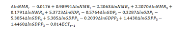
In the long run, LGDP has a negative impact on LNMR, while LGDPP has a positive impact on LNMR, and the coefficients are significant at the 1% level. In conclusion, I found out that LGDP and LGDPP have a symmetric impact on NMR in the long run-on average, ceteris paribus. The VECM fit the data very well overall, with an adjusted R squared of 97.7%; additionally, the F-statistics were significant at the 1% level.

Diagnostic check under NMR

The model’s post-estimation results revealed no serial correlation; error terms were normally distributed, with no heteroscedasticity based on the Breusch-Pagan- Godfrey test at 5%; and the VECM specification imposed 2-unit moduli, implying a high level of stability (Table 9).

Table 9: Neonatal mortality Rates VECM (Data 1954-2018)

Variables	Coefficient	Std. Error	t-Statistic	Prob.
ECT (-1)	-0.014009	0.003697	-3.789779	<0.001*
LNMR
LD.	0.989889	0.182500	5.424048	<0.001*
L2D.	-2.206255	1.564052	-1.410602	0.1672
L3D.	2.207011	1.563942	1.411185	0.1670
L4D.	0.179099	0.252715	0.708698	0.4832
LGDP
LD.	5.372330	4.102797	1.309431	0.1989
L2D.	-5.376400	4.102640	-1.310473	0.1986
L3D.	-0.328703	0.251977	-1.304497	0.2006
L4D.	-5.391813	4.149732	-1.299316	0.2023
LGDPP
LD.	5.385482	4.149856	1.297751	0.2029
L2D.	-0.203926	0.178766	-1.140742	0.2617
L3D.	1.442991	1.642640	0.878458	0.3857
L4D.	-1.446025	1.642367	-0.880451	0.3846
Cons	0.017644	0.007611	2.318407	0.0264
R-squared	0.983543	Mean dependent var		-0.020638
Adjusted R-squared	0.977431	S.D. dependent var		0.011313
S.E. of regression	0.001700	Akaike info criterion		-9.681903
Sum squared Resid	0.000101	Schwarz criterion		-9.141383
Log likelihood	251.2066	Hannan-Quinn criter.		-9.476831
F-statistic	160.9079	Durbin-Watson stat		1.923443
Prob(F-statistic)	0.000000

Short-run causality

The VECM results revealed no short-run causality running from the lagged values of NMR; in particular, the current values of NMR tend to increase with neonatal mortality before 99%. Furthermore, there were no short-run causalities from lagged GDP and GDPP values to NMR because their coefficients were not significant at the 5% level, implying that there is no short-run causality from LGDP and LGDPP to LNM (Table 10).

Table 10: VECM with Johansen normalization restriction imposed

Beta	Coef.	Std. Err.	z	P>z
LNMR (-1)	1.0000	.	.	.
LGDP (-1)	1.0155	0.1049	9.6795	0.000
LGDPP (-1)	-1.1797	0.1998	-5.9061	0.000
Cons	-19.6917	.	.	.

Long-run causality

The VECM results showed an adjustment term of -0.014, suggesting that the previous year’s errors are corrected within the current year at a convergence speed of 1.4% annually, towards long-run equilibrium. Furthermore, it indicated long-run causality running from LGDP and LGDPP to LNMR.

In the short run (1–6 years), the majority of the neonatal mortality forecast error variances (over 89%) were explained by themselves, and only a very small percentage was explained by GDP and GDPP. This influence reduced with time to the extent that, between 10 and 15 years, the influence of GDPP on NMR became stronger and that of GDP remained weak all through the period (Table 11).

Table 11: VECM projection error Variance Decomposition of LNMR

Period (Years)	S.E.	LNMR	LGDP	LGDPP
1	0.001700	100.0000	0.000000	0.000000
2	0.004075	97.91209	1.393570	0.694340
3	0.007194	97.15839	1.209350	1.632262
4	0.010488	96.43193	0.580207	2.987866
5	0.013667	94.26186	0.658029	5.080107
6	0.016684	89.90393	1.688806	8.407265
7	0.019628	83.41279	2.999677	13.58754
8	0.022695	75.56837	3.619241	20.81239
9	0.026055	67.15857	3.348640	29.49279
10	0.029772	59.10897	2.638423	38.25261
11	0.033746	52.17818	2.089350	45.73247
12	0.037718	46.72443	1.964940	51.31063
13	0.041405	42.73652	2.264125	54.99935
14	0.044613	39.97626	2.919827	57.10391
15	0.047295	38.14498	3.918061	57.93695

Forecast of infant and neonatal mortality in Uganda

After assessing the forecasting powers of the models, predictions for infant and neonatal mortality in the long run up to 2035 based on the Vector Error Correction Model (VECM) were estimated since it proved to be more reliable in making long-term forecasts (Table 12).

Table 12: Forecast of Infant Mortality Rate (IMR) and Neonatal Mortality Rate (NMR)

Time period	Lower limits	IMR	Upper limits	Lower limits	NMR	Upper limits
2020	31.9	32.3	32.6	19.4	19.4	19.5
2021	30.5	31.2	31.9	18.7	18.8	19.0
2022	29.0	30.1	31.3	18.0	18.2	18.4
2023	27.6	29.2	30.9	17.3	17.6	17.9
2024	26.2	28.3	30.5	16.7	17.1	17.4
2025	25.0	27.5	30.2	16.2	16.7	17.1
2026	23.8	26.7	29.9	15.9	16.4	16.8
2027	22.7	25.16	29.4	15.7	16.2	16.7
2028	21.5	24.9	28.8	15.5	16.0	16.6
2029	20.3	23.9	28.1	15.2	15.16	16.4
2030	19.1	22.8	27.1	14.9	15.5	16.2
2031	17.9	21.6	26.0	14.5	15.2	15.9
2032	16.8	20.4	24.9	14.1	14.8	15.5
2033	15.16	19.3	23.7	13.7	14.4	15.1
2034	14.8	18.3	22.6	13.3	14.0	14.7
2035	13.9	17.3	21.5	12.9	13.6	14.3

Globally, there has been a steady decline in NMR figures over the years, particularly in Uganda; however, this appears to have stalled in recent years, and this trend of slow decline is expected to continue during the lifespan of the Sustainable Development Goals if nothing is done. As presented in Figure 3,

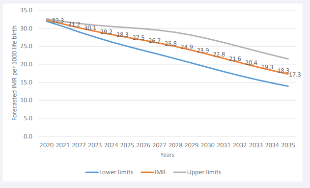
Figure 3: Forecast of NMR up to 2035 using VECM

we applied the suitable prediction model (VECM) after a deeper investigation of its capability to conduct both the short- and long-term forecast. It was observed that by 2035, Uganda will have about 17 deaths per 1,000 live births.Results presented in Figure 4 show that the decline of NMR will continue to slow over the next 15 years.

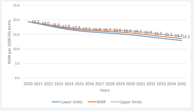
Figure 4 Forecast of NMR up to 2035 using VECM

The projections here presented provide an indication of where the health practitioner should focus. If the goal of eradicating infant mortality is to be realized, more emphasis should be placed on new-born life throughout the country.

My analysis of the association between IMR, NMR, and GDP as well as GDPP showed a significant negative correlation; as the GDP and GDPP of the country increase, the resources available for investment in the health subsector increase, thereby increasing access to improved health services by citizens, which in turn increases the survival rate of infants. In a nutshell, the response of LIMR to a one standard deviation (SD) shock (innovation) in LGDP remained steady at about zero in the first five years and increased slightly in the subsequent five years; however, beyond 10 years, LIMR rose quickly as compared to the previous period and it remains in the positive region. That is, shocks to LGDP will have a positive impact on LIMR in both the short and long run. According to the coefficients (pv=0.05), the long run equation also revealed that LGDP has a negative effect on IMR while GDPP has a positive effect on infant mortality. In a nutshell, LGDP and LGDPP have a symmetric effect on LIMR in the long run, on average, ceteris paribus. This result was consistent with the findings of Khan et al., (2019), who forecasted IMR for Asian countries using the log-log regression and ARIMA models, which included GDP and infant mortality. Their studies showed that IMR and GDP did correlate well.

Other studies also looked at the effect of economic recession measured in terms of GDP on infant and maternal mortality [4]. The study suggested that recessions do have a negative association with maternal and infant outcomes, particularly in the earlier stages of a country’s development, although the effects vary widely across different systems. Almost all of the 20 least wealthy countries have suffered a reduction of 10% or more in GDP per capita in at least one of the last five decades. Economic development seems to provide an important context that should be coupled with broader health-system interventions. The study noticed that there is a significant two-way causality between IMR and GDPP and a one-way causal effect from IMR to GDP. Interestingly, it was then clear that GDP only causes IMR through GDPP. There was a strong relationship between health outcomes (such as IMR and NMR), and GDP, just like GDPP, which could be due to the level of human capital dependency and the higher marginal effect of health spending on LIC and LMIC. This was in agreement with the research conducted by Amiria and Gerdtham [6], who found that there was a stronger relationship because the effects of GDP on health are stronger in LIC and LMIC compared to HIC and UMIC, while in contrast, the effects of health on GDP are stronger in HIC and UMIC compared to LIC and LMIC.

In a study that compared the SAARC bloc’s GDP per capita, health spending, and education spending to its human development index from 1990 to 2016, panel data analysis revealed that the HDI of SAARC has been rising with upward structural breaks [10]. Between 1990 and 2016, the HDI was inversely correlated with spending on health and education and positively correlated with GDP per capita. They have at least one cointegrating equation and significant long-run causalities from GDP per capita, health spending, and education spending to the SAARC human development index, but no immediate ones. Instead, there was a direct causal link between the human development index and the SAARC countries’ health spending [11].

While investigating the forecasting powers of different econometric models such as BVAR, VAR, and VECM to ascertain which of these models could best be employed in the short and long run, I discovered that BVAR and VAR models are best suited for short-run forecasts, while VECM yielded very convincing long-run forecast accuracy. The accuracy of these models was assessed in a 15-year out-of- sample forecast for both IMR and NMR based on root mean squared error (RMSE), mean absolute error (MAE), mean absolute percent error (MAPE), and the Theil inequality coefficient. Other results from the modeling of mortality in Australia using Bayesian Vector Autoregression (BVAR) showed how the Bayesian Vector Autoregressive (BVAR) models improve forecast accuracy compared to VAR models and quantify parameter risk, which is shown to be significant [10].

The supremacy of VECM follows the conclusion from similar studies in Australia by Kurniasih et al.[10], they said that in order to guarantee the existence of long-run correlations between mortality rate improvements, they suggested a large vector autoregressive (VAR) model fitted on the differences in the log-mortality rates. In addition, the study by Arnold & Sherris [15], applied VECMs to cause-of-death mortality rates to assess the dependence between these competing risks in Switzerland. The analysis confirms the existence of a long-run stationary relationship between these five causes. Zhou et al. [14], investigated how the modeling of the stochastic factors may be improved by using a Vector Error Correction Model. These findings support the notion that VECM provides more reliable long-term forecasts.

Macroeconomic variables such as GDP and GDPP are important components that can be used to predict infant mortality in both the short and long run. The analysis results showed that the short run forecasts could be made using univariate time series (ARIMA), since for both NMR and IMR, the majority of the forecast error variance can be explained by themselves, and this was also further alluded to in the short run coefficient of the VECM. Although long- run forecasts of both IMR and NMR can be done more accurately and successfully using VECM than VAR and BVAR models.

Although GDPP had a longer-term advantage over GDP on measures of infant mortality (IMR), GDPP had a longer- term advantage over GDP on these measures. In general, the ability to forecast IMR over the long term more accurately with GDP and NMR more effectively with GDPP Since the nation’s GDP is collective in nature, it was only natural that it would favor infants in terms of infrastructure and social service supply in the nation that supports baby survival. The GDPP, on the other hand, offers the closest amount of resources at the individual level that can meet the demands of children.

The study findings revealed that VAR or BVAR perform best in making short run forecast as compared to VECM based on RMSE, and hence for future long-run forecasts, there is a need to use VECM. In general, the ability to forecast IMR over the long term more accurately with GDP and NMR more effectively with GDPP Since the nation’s GDP is collective in nature, it was only natural that it would favor infants in terms of infrastructure and social service supply in the nation that supports baby survival. The GDPP, on the other hand, offers the closest amount of resources at the individual level that can meet the demands of children.

We thank the World Bank and UNICEF for providing us data. We thank Makerere University for approving the study.

OB: Conceptualization, Data Curation, Investigation, Methodology, Project Administration, Software, Writing original draft, and visualization. BO: Formal Analysis, Validation, reviewing, and editing: ET: Software, Validation; SM: Formal Analysis, Data Curation.

All Authors declare that the information provided in the publication is authentic with not bias 

Data can be accessed through the World Bank and UNICEF website

1. Baraki A, Kedir H, Geda T. The impact of preventable neonatal encephalopathy and infections on neonatal mortality in developing countries. Int J Pediatr. 2020; 8: 72-79.
2. WHO (World Health Organization). Neonatal Mortality: The Silent Epidemic. Geneva: World Health Organization. 2017.
3. Khelfaoui M, Zougari S, Douma L. The impact of maternal education and economic factors on infant mortality in Uganda. J Development Economics. 2022; 87: 89-104.
4. Ensor T, Gafur S. The effect of GDP fluctuations on maternal and infant mortality rates in developing nations. J Health Economics. 2010; 22: 223-235.
5. UNICEF. Levels and Trends in Child Mortality: Report 2017. United Nations Children’s Fund. 2017
6. Arshia Amiria, Ulf-G Gerdtham. The causal effect of maternal and child mortality on GDP in high-income and upper-middle-income countries. Int J Health Economics Management. 2013; 13: 121-136.
7. Erdil E, Yildirim A. Granger-causality approach to examining GDP and health expenditures per capita. Applied Economics Letters. 2010; 17: 1151-1155.
8. Usman A. Application of ARIMA models to analyze newborn mortality trends in Nigeria. Int J Health Forecasting. 2019; 28: 171-182
9. Ogedi I. Comparison of ARIMA and other time series methods for forecasting neonatal mortality rates in Nigeria. Afr J Health Economics. 2022; 28: 59-73.
10. Kurniasih W. Evaluation of the accuracy of ARIMA, Holt-Winters, and the α-Sutte Indicator in forecasting mortality rates. Asian J Forecasting. 2018; 25: 205-218.
11. Bhowmik M. Relationship between GDP, health expenditure, and the Human Development Index in the SAARC region. J Development Studies. 2019; 17: 35-48.
12. IMF (International Monetary Fund). World Economic Outlook: Sub- Saharan Africa: Navigating Headwinds. Washington, DC. 2017.
13. Sulaiman T, Salleh M. Forecasting infant mortality in developing countries using the Vector Error Correction Model (VECM). J Health Economics. 2019; 19: 210-218.
14. Zhou H. Mortality rate modeling using VECM: An approach for improving forecast accuracy. J Forecasting. 2014; 33: 56-63.
15. Arnold F, Sherris J. Application of VECM in assessing cause-of-death mortality rates. J Population Health. 2013; 56: 459-478.
16. Siahanidou T. Analysis of IMR trends in Greece from 2004 to 2016 using VECM. Eur J Population. 2019; 35: 787-799.
17. Lin W, Lee C. Exploring the relationship between healthcare spending and life expectancy using VECM. Int J Public Health Economics. 2016; 49: 112-130.
18. Faye O. Assessing the relationship between health expenditure, GDP, and IMR in the Philippines using a Vector Autoregressive (VAR) model. Global Health Action. 2014; 7: 28-36.
19. Shannon R Lane. The impact of public health expenditure on national health outcomes: Observations from cross-country data. Am J Public Health. 2013; 12: 300-315.
20. Chung H, Muntaner C. The effect of income inequality on infant mortality across various countries. Am J Public Health. 2006; 96: 1780-1786.
21. Kholid H. Forecasting health outcomes in low-income countries using Bayesian VAR models. Int J Health Forecasting. 2019; 45: 168-182.
22. Elliott G, Rothenberg TJ, Stock JH. Efficient Tests for an Autoregressive Unit Root. J Econometrics. 1996; 64: 813-836.
23. Guibert L, Lopez B, Piette J. Forecasting mortality rates using Bayesian VAR: Improving forecast accuracy in uncertain environments. J Forecasting. 2019; 40: 290-302.
24. Dickey DA, Fuller WA. Likelihood ratio statistics for autoregressive time series with a unit root. Econometrica. 1981; 49: 1057-1072.
25. Fernández C. Comparison of VAR and BVAR models in forecasting macroeconomic variables. J Forecasting. 2018; 37: 529-546.
26. Danao M S. Statistical methods for time series analysis: Issues in regression and co-integration models. Economic J Southeast Asia. 2002; 24: 111-132.
27. Box GE P, Jenkins GM. Time Series Analysis: Forecasting and Control (2nd ed.). Holden-Day. 1990.
28. Dickey D A, Fuller W A. Distribution of the estimators for autoregressive time series with a unit root. J Am Statistical Association. 1979; 74: 427-431.
29. Sims CA. Macroeconomics and Reality. Econometrica. 1980; 48: 1-48.
30. Lane S R. The impact of public health expenditure on national health outcomes: A statistical analysis. J Public Health Policy. 2013; 34: 396-405.
31. Liao TF. Analysis of the relationship between health expenditures and health outcomes in China using Vector Autoregressive (VAR) models. Asian J Public Health. 2017; 37: 209-220.
32. Mishra S, Sahanaa R, Manikandan S. Forecasting IMR in India from 1971 to 2016 using ARIMA models. Int J Health Forecasting. 2019; 26: 123-126.