A Bivariate Mixed Model Approach in Characterizing the Evolution of Longitudinal Body Mass Index and Quality of Life Processes in Adolescents with Severe Obesity Following Bariatric Surgery: A 5-Year Follow-Up of the Teenlabs Cohort

Resmi Gupta; Jane Khoury; Todd M Jenkins; Shelley Ehrlich; Richard Boles; Marc P Michalsky; Thomas H Inge; Rhonda D Szczesniak

doi:10.47739/1033

A Bivariate Mixed Model Approach in Characterizing the Evolution of Longitudinal Body Mass Index and Quality of Life Processes in Adolescents with Severe Obesity Following Bariatric Surgery: A 5-Year Follow-Up of the Teenlabs Cohort

Research Article | Open Access | Volume 5 | Issue 1

Article DOI : https://doi.org/10.47739/2374-0116/1033

Resmi Gupta^* Jane Khoury Todd M Jenkins Shelley Ehrlich Richard Boles Marc P Michalsky Thomas H Inge Rhonda D Szczesniak

^1. Division of Biostatistics and Epidemiology, Cincinnati Children’s Hospital, Cincinnati, OH, USA

+ Show More - Show Less

Corresponding Authors

Resmi Gupta, Division of Biostatistics and Epidemiology, Cincinnati Children’s Hospital, Cincinnati, OH, USA, Tel: 513 803-2087;

Abstract

Obesity is identified as a major global health problem. Along with measuring Body Mass Index (BMI), the most common metric for defining weight status, health related quality of life (HRQol) has been accepted as a routine method to evaluate how body weight may be impacted by psychosocial factors. The objective of the current study is to characterize the joint association of change in longitudinal BMI and HRQol following metabolic and bariatric surgery and to examine the correlation between these two outcomes measured concurrently over time. We identified the optimal modeling strategy by comparing four models, all of which involved the covariance structures appropriate for correlated outcomes, BMI and HRQol in a repeated measures analysis. The bivariate random effects models performed better than the univariate random effects models. Moreover, bivariate models with composite covariate structures had better model fit compared to the bivariate random slope models. The bivariate models with composite covariate structures reflected that changes in HRQol (and BMI) were most significant during the first 6 months, a clinically useful window to monitor changes in post-operative HRQol and BMI, and if there might need to be additional interventions or at least, closer monitoring.

CITATION

Gupta R, Khoury J, Jenkins TM, Ehrlich S, Boles R, et al. (2020) A Bivariate Mixed Model Approach in Characterizing the Evolution of Longitudinal Body Mass Index and Quality of Life Processes in Adolescents with Severe Obesity Following Bariatric Surgery: A 5-Year Follow-Up of the Teenlabs Cohort. Ann Biom Biostat 5(1): 1033.

INTRODUCTION

The rate of obesity has increased among children and adolescents, producing worrisome trends with both immediate and long term health consequences. Recently published data from the World Health Organization indicate that the number of girls and boys with obesity worldwide increased tenfold from 1975 to 2016, from 11 million to 124 million [1]. The most popular measure to define weight status is body mass index (BMI), expressed as weight in kilograms divided by height in meters squared (kg/m2). Based on US dietary guidelines, healthy weight, overweight, and obese categories are defined as a BMI of 18.5-24.9, 25-29.9 and, ≥30 $Kg/m^{3}$ respectively. Based on these categories, the National Health and Nutrition Examination Survey showed that the national obesity rate among children and youth between 2 to 19 years is 18.5% [2]. Although recent studies have reported decreased in obesity prevalence among younger children, in 2011 2012, 16.9% of children in the US were classified as obese, with prevalence being highest at ages 12-19 and lowest at ages 2-5 years. The modern definition of severe obesity, i.e. obesity classification of class II or higher, includes individual with BMI ≥120% of the 95th percentile.

High BMI in childhood is associated with increased risk of cardiovascular disease, type 2 diabetes mellitus and premature death [3] later in life. In addition to the physical consequences, obesity is associated with psychosocial disability and decreased quality of life [4]. There is an increasing recognition of the association between BMI and health related quality of life [5] (HRQol). HRQol is a multi-dimensional concept capturing the dimensions of physical functioning and psychological and social well-being, and is considered a very important patient-relevant outcome [6]. In recently published studies, bariatric surgery has been shown to be significantly effective for weight loss among adolescents [7]. A recent study showed improvement in HRQol among severely obese children after intervention with metabolic and bariatric surgery [8]. BMI and HRQol are two important metrics used to comprehensively evaluate the impact of treatment of obesity on adolescents. When collecting BMI and HRQol concurrently over time, correct modeling of these two variables together may produce more precise estimates of the longitudinal BMI and HRQol changes, and provide additional insight into the synergistic effects of patient’s weight loss and their psychosocial wellbeing following metabolic and bariatric surgery.

In multivariate longitudinal data, multiple response variables, such as BMI and HRQol, are simultaneously measured over time on the same individuals. Often these concurrently measured multiple outcomes are correlated, and modeling them separately and drawing conclusions based on the separate models can produce inefficient results and misleading conclusions [9]. These shortcomings are the result of using the separate models which do not take into consideration the correlation between the two outcomes. The widely used univariate models, meant to assess a single outcome, include mixed effects models with subject specific random effects as proposed by Laird and Ware [10], Harville [11], and structured covariance models as proposed by Jennrich and Schluchter [12]. These models often include one or more random effects and allow separate estimation of the between- and within subject variances. The extension of these models, with joint modeling of multiple outcomes was introduced by Sy, Taylor, Cumberland [13], which estimate the correlation between outcomes in addition to subject specific random effects; thus, this approach allows for a more realistic assessment of how these processes behave jointly over time.

The purpose of this study is to characterize the joint association of longitudinally measured BMI and HRQol following weight loss surgery and to examine the correlation between these two outcomes measured concurrently over time. The proposed bivariate linear mixed effects model will be used to estimate the correlation between the two aforementioned outcomes in addition to providing insights on sources of variation in the data. Furthermore, a joint modeling approach may identify clinically vulnerable points in time with respect to changes in weight dynamics and HRQol, thereby allowing clinicians to intervene when an adolescent is at greatest risk of a poor outcome.

DATA SOURCES: TEEN-LABS COHORT

The Teen Longitudinal Assessment of Bariatric Surgery (Teen-LABS) study methodology has been previously described in detail elsewhere [14,15]. In short, a total of 242 adolescents, age ≤19 years, were enrolled in this prospective, observational study designed to collect standardized clinical and laboratory data on adolescents undergoing bariatric surgery between March 2007 and February 2012 in five US clinical centers. The majority of subjects were female (75.6%) and white (72.2%); most underwent Roux-en-Y gastric bypass (RYGB; 66.5%) followed by vertical sleeve gastrectomy (VSG; 27.7%) and laparoscopic adjustable gastric banding (LAGB 5.8%). Due to the relatively small number of subjects undergoing LAGB, this group (n=14) was excluded from the analysis. Our analysis focused on 5 years of follow up of 242 subjects with data collection at baseline, 6 months, 12 months, 24 months, 36 months, 48 months, and, 60 months.

STATISTICAL METHODS

We define a general bivariate linear mixed model which includes; subject specific random effects, a correlated time process, and measurement error. Specifically, Let $Y_{i}=\begin{bmatrix} Y_{i1}\\ Y_{i2} \end{bmatrix}$ be the response vectors of subject i, with $Y_{ik}$ as the kth response vector, (k=1,2 corresponding to BMI and HRQol outcomes respectively) for the Teen-Labs cohort with $n_{iBMI}=n_{iHrQql}=n_{i}$ . Each response vector was obtained from the ith subject at baseline, 6 month, 12 month, 24 month, 36 month, 48 month, and 60 month. If BMI and HRQol are independent, the two univariate models can be written as:

$Y_{i1}=\beta _{1}X_{i1}+\gamma _{i1}Z_{i1}+\delta _{i1}+\varepsilon _{i1}----\left ( 1 \right )$

$Y_{i2}=\beta _{2}X_{i2}+\gamma _{i2}Z_{i2}+\delta _{i2}+\varepsilon _{i2}-----\left ( 2 \right )$

$\gamma _{i1}\sim N\left ( 0,\tau _{1} \right ); \gamma _{i2}\sim N\left ( 0,\tau _{2} \right ); \delta _{i1}\sim N\left ( 0,\upsilon _{i1} \right ); \delta _{i2}\sim N\left ( 0,\upsilon _{i2} \right );$

$\varepsilon _{i1}\sim N\left ( 0,\sigma _{si1}^{2}I_{ni} \right ); \varepsilon _{i2}\sim N\left ( 0,\sigma _{si2}^{2}I_{ni}\right );$

where $Y_{i1}$ and $Y_{i2}$ consist of vectors of all time points corresponding to BMI and HRQol respectively. $\beta _{k}$ is a $p_{k}$ vector of fixed effects, $X_{ik}$ is a $n_{i}\times p_{k}$ design matrix of traditional covariates, $Z_{ik}$ and $\gamma _{ik}$ correspond to design matrix and subject specific $q_{i}\times 1$ parameter vectors for random effects, $\delta _{ik}$ is a vector of correlation arising from multiple measurements from the same subject, and, $\varepsilon _{ik}$ represents the measurement error associated with the kth (k=1, 2) response vector.

To take into account the correlation between BMI and HRQol, the above two equations can be combined into a single equation to produce a bivariate linear mixed effects model:

$Y _{i}=\beta X_{i}+\gamma _{i}Z_{i}+\delta _{i}+\varepsilon _{i}-----\left ( 3 \right )$

$\varepsilon _{i}\sim N\left ( 0,\Sigma_{i} \right );\gamma _{i}\sim N\left ( 0,\Sigma_{\tau } \right );\delta _{i}\sim N\left ( 0,\upsilon _{i} \right )$

$\beta =\begin{bmatrix} \beta_{1} \\ \beta_{2} \end{bmatrix},X_{i}=\begin{bmatrix} X_{i1} &0 \\ 0 & X_{i2} \end{bmatrix},Z_{i}=\begin{bmatrix} Z_{i1} & 0\\ 0 & Z_{i2} \end{bmatrix},\gamma _{i}=\begin{bmatrix} \gamma _{i1}\\ \gamma _{i2} \end{bmatrix},\delta _{i}=\begin{bmatrix} \delta _{i1}\\ \delta _{i2} \end{bmatrix}$

In equation (3) above, $\gamma _{i}$ represents the subject-specific random effects corresponding to the BMI and HRQoL processes. For each subject, the covariance matrix of $\gamma _{i}$ can be written as $\Sigma _{\tau }=\begin{bmatrix} \sigma _{\gamma _{1}}^{2} & \sigma _{\gamma_{1} \gamma_{2} }\\ \sigma _{\gamma_{1} \gamma_{2} }& \sigma _{\gamma _{2}}^{2} \end{bmatrix}$ Moreover, the covariance matrix of the measurement error in equation (3), $\varepsilon _{i}$ , can be defined by $\Sigma_{i}= \Sigma \bigotimes I_{n_{i}}$ where $\bigotimes$ denotes a Kronecker product and $\Sigma =\begin{bmatrix} \sigma _{\varepsilon \left ( BMI \right )}^{2} &0\\ 0& \sigma _{\varepsilon \left ( HRQoL \right )}^{2} \end{bmatrix}$ . In equation (3) $\delta _{i}$ denotes a $2n_{i}$ vector of the bivariate visit process and is assumed to have a compound symmetric covariance matrix. The covariance structure for the bivariate visit process is given by $\begin{bmatrix} \sigma _{\upsilon _{1}}^{2} &\sigma_{\upsilon _{1}\upsilon _{2}}\\ \sigma_{\upsilon _{2}\upsilon _{1}}& \sigma _{\upsilon _{2}}^{2} \end{bmatrix}$ .With the assumption that $\varepsilon _{i}$ , $\gamma _{i}$ and $\delta _{i}$ are mutually independent, and the total variability of $Y_{i}$ can be written as, $Variance\left ( Y_{i} \right )=Z_{i}\tau _{i}Z_{i}^{T}+\upsilon _{i}+\Sigma _{i}$

Taking into account both repeated factors (response variables and visit), the bivariate composite covariance matrix can be specified for each of the repeat factors, i.e., the covariance model between BMI and HRQol within a visit, and the covariance model across the visit, and is given by:

$\begin{bmatrix} \sigma _{\varepsilon \left ( BMI \right )}^{2} &\sigma _{BMI,HRQoL}\\ \sigma _{HRQoL,BMI}& \sigma _{\varepsilon \left ( HRQoL \right )}^{2} \end{bmatrix}\bigotimes \begin{bmatrix} \sigma _{\upsilon _{1}}^{2} &\sigma_{\upsilon _{1}\upsilon _{2}}\\ \sigma_{\upsilon _{2}\upsilon _{1}}& \sigma _{\upsilon _{2}}^{2} \end{bmatrix}$

with respect to the Teen-Labs cohort, as seen in figure 1, there was a sharp decline in BMI and an increase in HRQol from baseline to 6 months post-surgery, and the average evolution was relatively stable over time after 6 months [16].

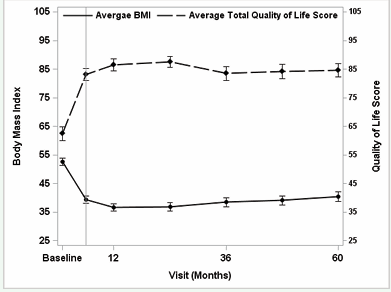
Figure 1: Mean and 95% confidence interval of body mass index and health related quality of life over time.

In order to capture the slope intensity before and after 6 months, we used a piecewise linear regression with a knot at 6 months in the regression models. We compared four models with two different types of covariance structures, random effects, and, compound symmetry in both univariate and bivariate modeling structures. The notation of each model is given below:

(i) Univariate models with two random slopes and a measurement error for each of the response variable, BMI and HRQol.

$Y_{i1}=\beta _{11}\left ( t_{i}\wedge \Psi \right )+\beta _{12}\left ( t_{i}- \Psi \right )I_{t_{i}\geq \Psi }+\beta _{13}\left ( age \right )_{i}+\beta _{14}\left ( gender \right )_{i}+\beta _{15}\left ( race \right )_{i}+\gamma _{11i}\left ( t_{i}\wedge \Psi \right )+\gamma _{12i}\left ( t_{i}- \Psi \right )I_{t_{i}\geq \Psi }+\varepsilon _{i1}------\left ( 4 \right )$ $Y_{i2}=\beta _{21}\left ( t_{i}\wedge \Psi \right )+\beta _{22}\left ( t_{i}- \Psi \right )I_{t_{i}\geq \Psi }+\beta _{23}\left ( age \right )_{i}+\beta _{24}\left ( gender \right )_{i}+\beta _{25}\left ( race \right )_{i}+\gamma _{21i}\left ( t_{i}\wedge \Psi \right )+\gamma _{22i}\left ( t_{i}- \Psi \right )I_{t_{i}\geq \Psi }+\varepsilon _{i2}------\left ( 5 \right )$

where $\beta _{k1}$ is the first slope from baseline to the 6 month visit, $\beta _{k2}$ is the second slope from the 6 month visit through 60 months. The parameter $\Psi$ equals the 6 month time point; $t_{i}\wedge \Psi$ denotes the minimum between $t_{i}$ and $\Psi$ .Moreover,??????? the subject specific random effects before the 6 month visit, and after the 6 month visit are given by $\gamma _{ik}$ . The measurement errors of the two response variables (BMI and HRQol) are given by $\varepsilon _{i1}$ and $\varepsilon _{i2}$ .

(ii) Bivariate model with random effects. With respect to the variance-covariance matrix, the equations (4) and (5) can be written as:

$\begin{bmatrix} \gamma _{11i}\\ \gamma _{12i}\\ \gamma _{21i}\\ \gamma _{22i} \end{bmatrix}\sim N\left [ \left [ 0_{\sim } \right ],\Sigma _{\gamma } \right ];$ $\Sigma _{\gamma }=\left [ \begin{bmatrix} \alpha _{BMI\left (before 6 mo \right )}^{2} & \alpha _{BMI\left (before 6 mo \right )}\alpha _{BMI\left (after 6 mo \right )} &\alpha _{BMI\left (before 6 mo \right )} \alpha _{HRQoL\left (before 6 mo \right )} & \alpha _{BMI\left (before 6 mo \right )} \alpha _{HRQoL\left (after 6 mo \right )}\\ \alpha _{BMI\left (after 6 mo \right )} \alpha _{BMI\left (before 6 mo \right )}& \alpha _{BMI\left (after 6 mo \right )}^{2} & \alpha _{BMI\left (after 6 mo \right )} \alpha _{HRQoL\left ( before 6 mo \right )}& \alpha _{BMI\left (after 6 mo \right )} \alpha _{HRQoL\left ( after 6 mo \right )} \\ \alpha _{HRQoL\left (before 6 mo \right )} \alpha _{BMI\left ( before 6 mo \right )} & \alpha _{HRQoL\left (before 6 mo \right )} \alpha _{BMI\left ( after 6 mo \right )} & \alpha _{HRQoL\left (before 6 mo \right )}^{2}&\alpha _{HRQoL\left (before 6 mo \right )} \alpha _{HRQoL\left ( after 6 mo \right )} \\ \end{bmatrix} \right ]$

(iii) Univariate model with compound symmetry. The model for each response variable, BMI and HRQol are expressed as:

$Y_{i1}=\beta _{11}\left ( t_{i}\wedge \Psi \right )+\beta _{12}\left ( t_{i}- \Psi \right )I_{t_{i}\geq \Psi }+\beta _{13}\left ( age \right )_{i}+\beta _{14}\left ( gender \right )_{i}+\beta _{15}\left ( race \right )_{i}+\gamma _{1i}+\varepsilon _{i1}------\left ( 6 \right )$ $Y_{i2}=\beta _{21}\left ( t_{i}\wedge \Psi \right )+\beta _{22}\left ( t_{i}- \Psi \right )I_{t_{i}\geq \Psi }+\beta _{23}\left ( age \right )_{i}+\beta _{24}\left ( gender \right )_{i}+\beta _{25}\left ( race \right )_{i}+\gamma _{2i}+\varepsilon _{i2}------\left ( 7 \right )$

(iv) Bivariate composite covariance model. With Kronecker [17] product , the covariance matrix for the between BMI and HRQol processes with knots at 6 month , and a compound symmetry covariance structure for the visit process, equations (6) and (7) can be expressed as:

$\begin{bmatrix} \gamma _{i1}\\ \gamma _{i2} \end{bmatrix}\sim N\begin{bmatrix} \begin{bmatrix} 0\\ 0 \end{bmatrix} & ,\upsilon _{i} \end{bmatrix} and \upsilon _{i}=\Sigma \gamma \bigotimes \begin{bmatrix} 1 & \rho & ..... &\rho \\ \rho & 1 & ..... &\rho \\ \rho & \rho & ...... &1 \end{bmatrix}$

where $\Sigma \gamma$ denotes the covariance matrix between the two outcome measures, BMI and HRQol, and the $\rho$ s denote the correlation due to the visit process. The univariate and bivariate random effects models were nested, and hence compared using the log likelihood [18]. Model comparison for the non-nested models, the bivariate random effects and the bivariate composite covariance model was conducted using Akaike information criteria (AIC) [19] and Bayesian information criteria (BIC) [20]. The demographic information, age, race and sex were selected as covariates in all the models. All models were implemented using SAS 9.4.4 (SAS, NC).

RESULTS

A total of 228 subjects were analyzed in this study. Majority of subjects were female (n=171; 75%) and white (n=164; 72%). The median (interquartile range; IQR) BMI and HRQol were 51 (45-58) kg/m2 and 62 (50-75) respectively. Figure 1 depicts the trajectories of BMI and HRQol, measured concurrently over time. The mean change over time for both BMI and HRQol depicts a point of inflexion at 6 months. Given the non-linearity and non-constant measures over time, we included a knot at 6 months which allows us to estimate more precise subject specific random effects through separate curves before and after 6 months. The approach using knot placement for points of inflection has been described elsewhere [16]. Surgery types was initially included in the models but was dropped later due to lack of statistical significance. Table 1 shows that the bivariate random effects model was significantly better compared to using two separate univariate random effects models (-2LogLikelihood = -16692, vs -17234; likelihood ratio test = 542 with 2 degrees of freedom, p<0.01 ; and, -16692, vs -17083; likelihood ratio test =380 with 2 degrees of freedom, p<0.01).

Table 1: Model fit estimates for the four models tested with respect to different covariance structures.
Models	-2Log-likelihood	Number of parameters	AIC	BIC
Univariate model with two random slopes	-17234	9	17254	17289
Bivariate model with two random slopes	-16692	11	16716	16757
Univariate model with compound symmetry	-17083	10	17105	17142
Bivariate composite covariance model	-16625	9	16633	16680
AIC: Akaike information criteria; BIC: Bayesian information criteria

Moreover, the bivariate composite model incorporating a compound symmetry visit process was better than the bivariate random effects model (AICBIV(Comp) = 16633 vs AICBIV(RS) = 16716; BICBIV(Comp) = 16680 vs BICBIV(RS) = 16757).

With a knot at 6 months, the bivariate random effects model allows us to estimate the correlation matrices between individual slopes for each variable, BMI and HRQol (Table 2).

Table 2: Estimated correlation matrix of bivariate mixed effects models with two random slopes.
	First slope of BMI	First slope of QOL	Second slope of BMI	Second slope of QOL
First slope of BMI	1
First slope of QOL	-0.65	1
Second slope of BMI	0.26	0.31	1
Second slope of QOL	0.27	0.06	-0.70	1

Briefly, the correlations between the slopes of the two measures, BMI and HRQol at the same time period , $\rho \hat{}_{BMI,HRQoL}$ before 6 months = -0.65; , $\rho \hat{}_{BMI,HRQoL}$ after 6 months = -0.70). These results were expected because of the underlying relationship between two variables following surgery. Moreover, the second slope of BMI was moderately correlated with the first slope of the same measures ( $\rho \hat{}_{BMI}$ (before 6 months, after 6 months) =0.26). However, low correlation was detected between first and second slope of HRQol measure ( $\rho \hat{}_{HRQoL}$ (before 6 months, after 6 months) =0.06). The HRQol is a weight-related quality of life metric, and hence it was anticipated to go hand-in-hand with weight changes.

The results for the best fitting model (bivariate with CS) are shown in Table 3.

Table 3: Analysis results of the bivariate linear mixed effects model with compound symmetry covariance matrix.
	BMI Est (SE) p-value		HRQol Est (SE) p-value		Correlation
Fixed
Rate of change (slope) before 6 mo	-3.7 (0.08)	<0.01	4.5 (0.21)	<0.01
Rate of change (slope) after 6 mo	0.18 (0.01)	0.07	-0.14 (0.03)	0.40
Age	0.19 (0.18)	0.58	-0.22 (0.24)	0.67
White vs others	-3.5 (1.59)	0.06	0.6 (2.11)	0.82
Male vs Female	3.4 (1.52)	0.02	2.2 (2.0)	0.27
Random
σ2(BMI)	131.2	<0.01
σ2(HRQol)	280.1	<0.01
σ (BMI,HRQol)	-5.2	<0.01
ρ(BMI)(tij)					0.87*
ρ(QOL)(tij)					0.62**
σ2ε(BMI)					0.07***
σ2ε(HRQol)					0.06****
EST: Estimate; : correlation between 2 consecutive measurements for BMI;: correlation between 2 consecutive measurement for QOL; : Measurement error for BMI; **: Measurement error for QOL

Males have higher BMI compared to females $\left ( \beta\hat{}_{Males}\left ( SE \right )=3.4\left ( 1.5 \right ),P=0.02 \right )$ . A greater rate of change is seen in BMI and HRQol before 6 month compared to after 6 month $\left ( \beta\hat{}_{BMI slope before6mo}\left ( SE \right )=-3.7\left ( 0.08 \right ),P< 0.01; \beta\hat{}_{HRQoL slope before6mo}\left ( SE \right )=4.5\left ( 0.21 \right ),P< 0.01; \beta\hat{}_{BMI slope before6mo}\left ( SE \right )=0.18\left ( 0.01 \right ),P= 0.07;\beta\hat{}_{HRQoL slope before6mo}\left ( SE \right )=-0.14\left ( 0.03 \right ),P= 0.4 \right )$

although for both measures the slopes after 6 months were not statistically significantly different from zero.

Output obtained from the bivariate composite covariance process provided estimates of variance-covariance matrices and the measurement errors of the two outcome measures. The variance measures of $BMI\left ( \sigma \hat{}_{BMI}^{2} =131.2\right )$ , $HRQoL \left ( \sigma \hat{}_{HRQoL}^{2} =280.1\right )$ and covariance between BMI and HRQol $\left ( \sigma \hat{}_{BMI,HRQoL} =-5.2\right )$ are all significantly different from 0 (Wald test, p<0.01), reflecting an underlying relationship between the two outcomes. The significant negative covariance estimate reflects that BMI and HRQol are inversely related, reflecting that the patients with higher variability in BMI exhibited less variability in HRQol measure. The parameter $\rho \hat{}$ signifies the estimated measurements of correlation between the two consecutive measures of BMI or HRQol $\left ( \rho \hat{}_{BMI\left ( t_{ij} \right )} =0.87;\rho \hat{}_{HRQoL\left ( t_{ij} \right )} =0.62\right )$ . The estimated model measurement errors were quite low for both BMI and HRQol??????? $\left ( \sigma _{S_{1\left ( BMI \right )}}^{2} =0.07; \sigma _{S_{\left ( BMI \right )}}^{2} =0.06Respectively\right )$ as shown in Table 3.

DISCUSSION AND CONCLUSION

In this assessment, we have considered four covariance models for modeling the covariance structures for correlated outcomes in a repeated measures analysis. With two longitudinal outcomes measured concurrently over time, we showed that the bivariate composite covariance models provided best fit among the models tested, namely, univariate and bivariate random effects models.

Understanding the evolution of the association between BMI and HRQOL jointly measured over time from the same subject could be a useful strategy to identify patient characteristics affecting patient wellbeing following weight loss surgery. The prevalence of childhood and adolescent obesity and in particular severe obesity, has been increasing, with a significant disease burden and costs, causing an important public health concern. Existing lifestyle interventions and medical treatments have shown only a modest effect, particularly for young people with severe obesity [21]. Over the past 20 years, metabolic and bariatric surgery has become an important treatment option for adults with severe obesity and is increasingly being offered to adolescents. The most commonly used method to assess the effects of weight loss surgery is BMI, a calculation that allows for adjustment of weight on the basis of height. In recent years, studies have been conducted establishing the importance of the association between BMI and health related quality of life outcomes in the adult population.

We modeled simultaneously the bivariate response of BMI and HRQol as functions of explanatory variables to evaluate whether a change in BMI over time is related to change in the HRQol score following weight loss surgery in Teen-Labs cohort. With two distinct slopes before 6 month and after 6 month following surgery, the bivariate random effects and bivariate composite covariance models provided better model fit compared to the univariate models.

Metabolic and bariatric surgery had the greatest impact on BMI and HRQol within six months for both BMI and HRQol. As reflected by the bivariate random effects model, the magnitude of correlations between changes in BMI and HRQol decreased over follow up. This information cannot be detected by the univariate models. The attractive feature of the bivariate model is that it allows simultaneous modeling of the two outcome measures BMI and HRQol, which is meaningful in the presence of correlation between the two measures. These results from bivariate linear mixed effects model enabled us to simultaneously explore the biological and psychological in determining the effects of bariatric surgery.

The bivariate linear mixed effects model with composite covariance structure presented here is conceptually appealing. With the composite covariance model incorporating the Kronecker product (unstructured x compound symmetry) to the two outcomes concurrently measured over time, we were able to fit the model more precisely. When one of the repeated factors has been measured more frequently than the other, the bivariate composite covariance structure may produce a convergence problem. In this study, one repeat factor, the number of visits, was much greater than the other repeat factor, the number of response variables, so a convergence problem emerged when we fitted the bivariate composite covariance model with an unstructured x unstructured covariance structure. This was because there were too many parameters to be estimated. Convergence model issues commonly occur in fitting the unstructured covariance model for unbalanced data [22].

For the Teen-LABS cohort study, the unstructured x compound symmetry assumption seemed to be more appropriate, because it allows arbitrary covariance between the two concurrent outcomes, BMI and HRQol, but assumes compound symmetry structure for observations within the same visit. Out of the four model tested, the bivariate composite model provided the best model fit and that changes in HRQol (and BMI) were most significant during the first 6 months, an attractive finding that a univariate model could not detect. It therefore seems to identify a clinically useful window to monitor changes in post-operative HRQol and BMI, and if there might need to be additional interventions or at least, closer monitoring. The composite covariance model can be easily fit using the SAS PROC Mixed procedure [23].

When the covariance structure is not known, a robust covariance structure as mentioned by Liang and Zeger [24] can be an alternative approach. However, there are some limitations for the practical use of this approach. The SAS PROC Mixed procedure cannot handle the robust covariance approach. The other SAS procedures, such as, PROC GENMOD or PROC Glimmix cannot handle composite covariance structure models. In this study, we used the compound symmetry covariance structure for the visit process because of unequal time intervals. Our model had a convergence problem when we applied the unstructured covariance matrix for the visit process in the composite model.

Modeling of variances and covariance’s requires a fair amount of data. The Teen-LABS data collection provides large numbers of repeated observations that can be used for these purposes. In this study we considered the bivariate response variables, BMI and HRQol, as functions of static explanatory variables. The model can be extended to consider time dependent covariates. Finally, changing the random effects distribution assumption and evaluating the model performance is an area of future study.